Get this post on pdf here.

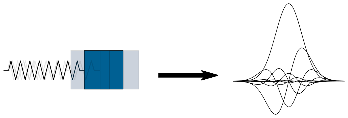
Quantization is the process that transforms a classical physical system into its quantum counterpart. As done by most physicists, quantization is quite ad hoc and not very rigorous. There’s a well-defined mathematical structure of classical mechanics (which is generalized into symplectic geometry), and there’s a well-defined structure of non-relativistic quantum mechanics (that of Hermitian operators on a Hilbert space); however, how one takes a classical object (be it state or observable) into its quantum counterpart is often not very clear.

In this post, we start a dive into one of the few ways mathematicians have tried to make quantization rigorous: geometric quantization. Its name comes from the fact that the quantization method arises somewhat naturally from the symplectic structure of phase space.

Before we look at geometric quantization, let’s look at quantization of classical phase space, as done by physicists. That way we can see what we want from a theory of quantization.

Consider the phase space of a particle, for simplicity in one spatial dimension. It has a position coordinate $q$ and a momentum coordinate $p$, and their Poisson bracket¹ is

\[\left\{q,p\right\} = \frac{\partial q}{\partial q}\frac{\partial p}{\partial p} - \frac{\partial p}{\partial q}\frac{\partial q}{\partial p} = 1.\]

Canonical quantization (or Heisenberg quantization) consists of turning $q$ and $p$ into Hermitian operators $\hat{q},\hat{p}$ on a Hilbert space $\mathcal{H}$, which satisfy the canonical commutation relations

\[[\widehat{q},\widehat{p}] = i\hslash.\]

So in brief, in physics we quantize by putting little hats on top of observables, declaring that they are Hermitian operators now, and imposing the canonical commutation relations.

More generally, we want to promote all functions $f(q,p)$ on phase space to Hermitian operators on some Hilbert space $\mathcal{H}$, in a way that respects the Poisson bracket. That is, for two functions $f$, $g$, we want their quantizations $\hat{f}$, $\hat{g}$ to satisfy

\[\left\{f,g\right\} \mapsto \frac{-i}{\hslash}[\hat{f},\hat{g}].\]

How do we obtain the quantization of such a function? Well, starting from the quantization of $q$ and $p$, we can quantize “all” functions that depend on only one of the variables $q$ or $p$, by “quantizing” each term of their Taylor expansion. For example, if we have a function $f(q)$, then its quantization is

\[f(q) = \sum_{n=0}^\infty a_nq^n \mapsto \hat{f} = \sum_{n=0}^\infty a_n\hat{q}^n.\]

In practice, quantizing all functions of only $p$ and only $q$ gets us quite far, since we are mostly interested in the Hamiltonian function, which is very often of the form

\[H(q,p) = \frac{p^2}{2m} + V(q),\]

where $V$ is a potential function that only depends on position. But what if the function we want to quantize depends both on $q$ and $p$ in a nontrivial way? Well... things get hairy then and there’s several, often non-equivalent, ways to deal with that.

Another question we have right now is... what is the Hilbert space $\mathcal{H}$? Here is where we connect with Schrödinger’s wave mechanics. The Hilbert space is $L^2(\mathbb{R})$, the space of square-integrable functions on the real line, and the operators $\hat{q}$, $\hat{p}$ have an explicit representation:

\[\begin{aligned} (\hat{q}\psi)(x) &= x\psi(x)\\ (\hat{p}\psi)(x) &= -i\hslash\frac{\mathrm{d}\psi}{\mathrm{d}x}.\end{aligned}\]

Following all these prescriptions, we have, for example, that the Hamiltonian of a free particle gets quantized as

\[\hat{H} = -\frac{\hslash^2}{2m}\frac{\mathrm{d}^2}{\mathrm{d}x^2}.\]

And the Hamiltonian of the harmonic oscillator with elastic constant $k$ gets quantized as

\[\hat{H} = -\frac{\hslash^2}{2m}\frac{\mathrm{d}^2}{\mathrm{d}x^2} + \frac{1}{2}kx^2,\]

where the second term is understood as multiplying by $x^2$.

Our wildest quantum dreams

Looking back on the previous section, we can try to fit all these into some axioms of quantization. What do we want from a quantization scheme?

We want a procedure that takes functions on phase space, and turns them into Hermitian operators on a Hilbert space. If we consider the phase space in $n$ dimensions, what we want then is a map $C^\infty(\mathbb{R}^n\times\mathbb{R}^n)\to \operatorname{Herm}(\mathcal{H})$, which we denote as $f\mapsto \hat{f}$. The first obvious condition is that it should turn Poisson brackets into commutation relations (times $i\hslash$). We can express this as:

Axiom 1: For any pair of functions $f$, $g\in C^\infty(\mathbb{R}^n\times\mathbb{R}^n)$, we have the canonical commutation relations

\[[\widehat{f},\widehat{g}] =i\hslash\widehat{\left\{f,g\right\}}.\]

This axiom is not enough to give us the canonical commutation relations of $p$ and $q$: we need to ensure that the quantization of the constant function $1$ is precisely the identity $I$. We introduce this as a second axiom:

Axiom 2: The quantization of the constant function $1$ is the identity $I$:

\[\hat{1} = I.\]

Another axiom that is well needed is that the quantization scheme should be linear. This is an implicit assumption when we do canonical quantization!

Axiom 3: The quantization scheme is linear.

The next axiom is the one that tells us that we can quantize functions by quantizing their Taylor expansions in a term by term basis. In most cases, we don’t even need to go that far: we just want the quantization scheme to respect the polynomial algebra generated by functions! That is:

Axiom 4: For any function $f$ and all $n\in\mathbb{Z}$:

\[\widehat{(f^n)} = (\widehat{f})^n.\]

The last axiom, doesn’t show up explicitly in canonical quantization, but it implies that the quantization of the functions $p$ and $q$ are the standard ones on $L^2(\mathbb{R})$. This is a condition imposing the irreducibility of the representation of the algebra of functions on the Hilbert space:

Axiom 5: The only subspaces $W\subseteq \mathcal{H}$ that are stable under the action of all the quantizations of the position and momentum functions are $0$ and $\mathcal{H}$. That is to stay: if $\hat{q}(W)\subseteq W$ and $\hat{p}(W)\subseteq W$, then $W=0$ or $W=\mathcal{H}$.

By the Stone-Von Neumann theorem, this, along with the canonical commutation relations of $\hat{q}$ and $\hat{p}$, implies their standard representations in $L^2(\mathbb{R})$.

Our dreams shattered

Welp, it turns out that the axioms above are too much to ask of a quantization scheme. As an example, let’s consider the function $pq$. Remember that we don’t know how to quantize products of $p$ and $q$, but if we rewrite it as

\[pq = \frac{1}{2}((p+q)^2-p^2-q^2),\]

we know how to quantize all the terms on the right-hand side, using axioms 2 and 4:

\[\widehat{pq} = \frac{1}{2}((\hat{p}+\hat{q})^2 - \hat{p}^2-\hat{q}^2) = \frac{1}{2}(\hat{p}\hat{q}+\hat{q}\hat{p}).\]

So far, so good. In a similar fashion, we get

\[\widehat{p^2q^2} = \frac{1}{2}(\hat{p}^2\hat{q}^2+\hat{q}^2\hat{p}^2).\]

But here we run into trouble. From axiom 4, we should have

\[\widehat{p^2q^2} = \widehat{(pq)^2} = \widehat{pq}^2,\]

but

\[\widehat{pq}^2\neq \frac{1}{2}(\hat{p}^2\hat{q}^2+\hat{q}^2\hat{p}^2).\]

So the scheme is inconsistent! And it turns out (see Ali & Engliš) that many more inconsistencies between these axioms.

So... why isn’t this a big problem in physics? It’s because we don’t care about the whole Poisson algebra of $C^\infty(\mathbb{R}^{n}\times\mathbb{R}^n)$! In practice, we only care about quantizing certain specific functions on phase space: energies, momenta, etc. These have explicit expressions which are often polynomials of low degree in $p$ and $q$, without any cross-terms like $pq$, which are the ones that bring trouble. Even more, if we have cross-terms as in the angular momentum

\[\mathbf{L} = \mathbf{q}\times\mathbf{p} = (q_yp_z-q_zp_y)\mathbf{e}_x + (q_zp_x-q_xp_z)\mathbf{e}_y + (q_xp_y-q_yp_x)\mathbf{e}_z,\]

the factors $q_ip_j$ are actually commuting, since the canonical Poisson algebra is

\[\left\{q_i,p_j\right\} = \delta_{ij}.\]

So in the end thereis no trouble.

What is our objective, then?

We know that it’s impossible to find a quantization scheme satisfying all the axioms, so what is our goal? At the outset, we need to relax some conditions.

First, we will not try to quantize the entire Poisson algebra of smooth functions on phase space. Instead, we will focus on a (possibly very small) subalgebra of quantizable observables, which we call $\mathrm{Obs}\subset C^\infty(\mathbb{R}^n\times\mathbb{R}^n)$. Furthermore, we will not require Axioms 4 and 5 anymore, which seem to be the most restrictive.

And even better, we don’t have to focus on the standard phase space $\mathbb{R}^n\times \mathbb{R}^n$, but instead we can try to find a quantization scheme for any symplectic manifold.

The geometric viewpoint of canonical quantization

Let’s put our geometer hats on and go back to the canonical quantization of $M=\mathbb{R}^n\times\mathbb{R}^n$. We’ll do some half guessing, half reverse-engineering to try to find:

1. A subalgebra of quantizable observables $\mathrm{Obs}$,

2. a Hilbert space of quantum states $\mathcal{H}$,

3. and a quantization scheme $\mathrm{Obs}\to\operatorname{Herm}(\mathcal{H})$ satisfying axioms 1, 2, and 3,

which hopefully coincides with the standard canonical quantization. Along the way, we’ll also be thinking about how to write these ideas in a coordinate-free way, so that we can generalize to symplectic manifolds.

Our guiding light is the first axiom: For any pair of functions $f$, $g$ in our (still undetermined) space of observable functions, we want their quantizations to satisfy the commutation relations

\[[\widehat{f},\widehat{g}]= i\hslash\widehat{\left\{f,g\right\}}.\]

Even more, we expect the quantized operators to act somewhat like differential operators on a space of functions (wavefunctions). This rings a symplectic bell! Recall that any smooth function on a symplectic manifold $(M,\omega)$ has an associated Hamiltonian vector field $X_f$ defined as

\[\iota_{X_f}\omega = \mathrm{d}{f}.\]

These vector fields are indeed operators acting on functions, and furthermore, they satisfy

\[X_{\left\{f,g\right\}} = -[X_f,X_g],\]

Where $\{f,g\} = X_g[f]$ is the standard Poisson structure induced by the symplectic structure. This tells us that a naïve, but good, start for a quantization rule is

\[\hat{f} = -i\hslash X_f,\]

since then we have

\[[\widehat{f},\widehat{g}]= -\hslash^2[X_f,X_g]=\hslash^2X_{\left\{f,g\right\}} = i\hslash(-i\hslash X_{\left\{f,g\right\}}) = i\hslash\widehat{\left\{f,g\right\}}.\]

So axiom $1$ is satisfied, but not axiom $2$, since the Hamiltonian vector field associated to a constant function is just $0$, so we need to tweak the quantization scheme. The first dumb guess is to add a multiplication by the original function, i.e.

\[\hat{f} \overset{?}{=} -i\hslash X_f + f,\]

so we fix the problem that the quantization of $1$ is not $\mathrm{id}$. However, as we see in the gory details below, we break the commutation rules:

\[[\widehat{f},\widehat{g}]= i\hslash\left(\widehat{\left\{f,g\right\}} + \left\{f,g\right\}\right)\]

One way to fix this is by choosing a symplectic potential $\theta$ for the symplectic form $\omega$; i.e. a form that satisfies $-\mathrm{d}\theta = \omega$, and defining the quantization of an observable as

\[\hat{f} = -i\hslash X_f + f - \theta(X_f).\]

This tweaking goes back to Segal, 1960, but it is left unmotivated. It is very likely that it was obtained by educated guessing and trial-and-error. We show that it is a good quantization scheme in the gory details below.

How does this look like in $\mathbb{R}^{n}\times\mathbb{R}^n$? If we choose global coordinates $q^\mu$, $p_\mu$, the symplectic form is

\[\omega = \mathrm{d}{q}^\mu\wedge\mathrm{d}{p_\mu},\]

and the Hamiltonian vector field associated to a function $f\in C^\infty(\mathbb{R}^n\times\mathbb{R}^n)$ is

\[X_f = \frac{\partial f}{\partial p_\mu}\frac{\partial }{\partial q^\mu} - \frac{\partial f}{\partial q^\mu}\frac{\partial }{\partial p_\mu},\]

so that the Poisson bracket of two functions is

\[\left\{f,g\right\} = \frac{\partial f}{\partial q^\mu}\frac{\partial g}{\partial p_\mu} - \frac{\partial f}{\partial p_\mu}\frac{\partial g}{\partial q^\mu}.\]

A symplectic potential is given by the tautological form, which is defined in these coordinates as² \(\theta = p_\mu\mathrm{d}{q^\mu}.\) It is straightforward to show that this quantization scheme is explicitly

\[\hat{f} = -i\hslash\left(\frac{\partial f}{\partial p_\mu}\frac{\partial }{\partial q^\mu} - \frac{\partial f}{\partial q^\mu}\frac{\partial }{\partial p_\mu} \right) + f -p_\mu\frac{\partial f}{\partial p_\mu}.\]

Alright! So we’re done! Let’s see what happens to the coordinate functions. For the momenta $p_\mu$, we have

\[\hat{p}_\mu = -i\hslash\frac{\partial }{\partial q^\mu}.\]

Perfect! And for the positions $q^\mu$:

\[\hat{q}^\mu = i\hslash\frac{\partial }{\partial p_\mu} +q^\mu.\]

Ah fuck. It’s okay, we can fix it. In fact, there is nothing wrong here! You see, these are operators that have to act on some vector space. In canonical quantization, this is the space of complex-valued, square-integrable wavefunctions $L^2(\mathbb{R}^n)$, which consists of functions only of the $q$ variables! So the leftover term in $\hat{q}^\mu$ is actually zero, since the wavefunctions do not depend on $p$.

So our first attempt at a rigorous canonical quantization is the following:

1. The symplectic manifold is $\mathbb{R}^n\times\mathbb{R}^n$, with the standard symplectic structure.

2. The quantum state space is $L^2(\mathbb{R}^n)$, defined in the $q$ variables only.

3. The quantization of an observable $f\in\mathbb{C}^{\infty}(\mathbb{R}^n\times\mathbb{R}^n)$ is given by

   \[\hat{f} = -i\hslash X_f + f - \theta(X_f),\]

   where $\theta$ is the tautological form.

Of course, there are a few problems there if we try to go to general symplectic manifolds. First of all, there might not be a global choice of a symplectic potential, so the quantization of an observable might change as we move around the manifold. In fact, even locally the choice of a potential is not unique. No bueno. Furthermore, in a general manifold there isn’t a canonical separation of position and momenta: we just have an even amount of coordinates. So how do we make a coordinate-free definition of a function depending “only on the $q$ coordinates”?

Let’s tackle the first problem.

Gauge symmetries

The quantization of observables requires a choice of a symplectic potential. In the case of canonical quantization, there is a canonical choice given by the tautological form.³ But in the general case of symplectic manifolds,⁴ symplectic potentials exist at best locally, and the choice is far from unique. Can we get a quantization of observables that is independent from the choice of symplectic potential?

Suppose that we have two symplectic potentials $\theta$ and $\theta’$, defined locally on some open sets $U$ and $U’$, such that on the intersection $U\cap U’$ we have

\[\theta' = \theta + \mathrm{d}{u}.\]

This, of course, changes the quantization of an observable:

\[\hat{f}'= -i\hslash X_f + f - \theta'(X_f) = \hat{f} - \mathrm{d}{u}(X_f).\]

Consequently, the action of $\hat{f}’$ on a wavefunction $\psi$ will differ from that of $\hat{f}$. But all is not lost! In quantum mechanics, we don’t really care about wavefunctions, but instead the expectation values of observables:

\[\left\langle\psi\middle\vert\hat{O}\psi\right\rangle.\]

That means that if we change the observables and the wavefunctions such that the expectation values are preserved, then all is well!

I’ve discussed this idea previously in another post, but the gist is the following. If we change the wavefunction as

\[\psi' = e^{\frac{i}{\hslash}u}\psi,\]

then it is straightforward to check that the action of $\hat{f}’$ on $\psi’$ satisfies

\[\hat{f}'\psi' = (\hat{f}\psi)'.\]

That is, if we transform the operator and apply it to the transformed wavefunction, we get the same thing as applying the original operator to the original wavefunction and then transforming. Furthermore, we see that the operators change as

\[\hat{f}' = e^{\frac{i}{\hslash}u}\hat{f}e^{-\frac{i}{\hslash}u},\]

and so the expectation values are preserved exactly:

\[\left\langle\psi'\middle\vert\hat{f}'\psi'\right\rangle = \left\langle\psi\middle\vert\hat{f}\psi\right\rangle.\]

This suggests that we should think of the wavefunction as a section of a line bundle $L$ that has transition functions $e^{-\frac{i}{\hslash}}$, and that the operators act on this space of sections. Furthermore, if we write the action of $\hat{f}$ as

\[\hat{f}\psi = -i\hslash\left(\mathrm{d}{\psi} -\frac{i}{\hslash}\theta\cdot\psi\right)(X_f) + f,\]

we see that the term in brackets is precisely the local expression of a connection (or covariant derivative) on $L$:

\[\nabla = \mathrm{d}-\frac{i}{\hslash}\theta,\]

whose curvature is precisely

\[R^\nabla = -\frac{i}{\hslash}\mathrm{d}{\theta} = \frac{i}{\hslash}\omega.\]

We call the bundle $L$ the prequantum line bundle, and from its curvature we can see that its Chern class is

\[c_1(L) = \frac{1}{2\pi\hslash}[\omega].\]

With this in mind, we can think of the state space as the set of sections of the prequantum line bundle, and the quantization of a function $f\in C^\infty(M)$ is

\[\hat{f}\psi = -i\hslash\nabla_{X_f}\psi + f\psi.\]

The first obstruction

It turns out that having a line bundle $L$ with a connection whose curvature is $\frac{i}{\hslash}\omega$ imposes a restriction on the symplectic form. Namely, we require $\frac{1}{2\pi\hslash}[\omega]$ to be an integral cohomology class.

Let’s see this briefly. Consider a cover $\{U_j\}$ of $M$, where each $U_j$ is contractible and such that on each $U_j$ we have symplectic potentials $\theta_j$. Then on intersections, we can define the transition functions $u_{ij}:U_i\cap U_j\to \mathbb{C}$ satisfying

\[\mathrm{d}u_{ij} = \theta_i - \theta_j.\]

As we saw above, the transition functions of the prequantum line bundle $L$ are of the form $\exp(\frac{i}{\hslash}u_{ij})$, and so they must satisfy the cocycle conditions

\[\exp(\frac{i}{\hslash}(u_{ij}+u_{jk}+u_{ki}))=1,\]

which means that the functions $z_{ijk}:U_i\cap U_j\cap U_k\to \mathbb{C}$ defined as

\[z_{ijk} = \frac{1}{2\pi\hslash}(u_{ij}+u_{jk}+u_{ki})\]

are integer-valued, and so must be constant. The collection of these $z$ functions forms a Čech 2-cocycle, and its cohomology class $[z]\in\check{H}^2(M,\mathbb{Z})$ agrees precisely with the class $\frac{1}{2\pi\hslash}[\omega]$.⁵

This integrality condition is satisfied trivially in the case of $\mathbb{R}^{n}\times \mathbb{R}^{n}$, since the symplectic form is exact and thus its cohomology class is zero. In fact, in the case of any cotangent bundle, the canonical symplectic form is exact and so its cohomology class is zero. This is good news! This tells us that we can at least attempt to quantize classical systems.

We say that a symplectic manifold that satisfies the integrality condition is prequantizable.

Reducing the number of variables: Polarizations

Now that we’ve dealt with the problem that the quantization of a function depended on the choice of a symplectic potential, we move on to discuss the other problem: How do we generalize the idea of a function depending only on “half the number of variables” to a symplectic manifold, where the choice of (Darboux) coordinates is not canonical?

Let’s look at the specific example of $\mathbb{R}^n\times \mathbb{R}^n$ and let’s try to see how to take it to a coordinate-free context. We said that the true set of wavefunctions was $L^2(\mathbb{R}^n)$, functions that depend only on the position coordinates $q^\mu$ but not on the momenta $p_\mu$.

In a symplectic manifold, we don’t have a consistent choice of every $q^\mu$ and $p_\mu$ globally. However, we can relax this and simply ask a splitting of the local coordinates into $q$’s and $p$’s in such a way that they don’t get mixed together as we move around the manifold. Maybe when we change charts, the $q$’s get mixed among themselves, maybe the $p$’s get mixed among themselves, but we don’t have $q$’s turning into $p$’s or vice-versa. This way, we can have a notion of a function being “independent from the $p$’s” without actually having globally-defined symplectic coordinates. We just need a notion of “directions along the momenta” at each point, and so a function whose derivative vanishes along those directions will be independent of the momenta.

How do we achieve this in practice? At each point $x\in M$, we want to choose a half-dimensional subspace $P_x$ of the tangent space $T_xM$. This half-dimensional subspace will be the space of “momentum directions”, but what does that mean exactly? How can we make sure that we don’t introduce “position directions” in $P_x$? Well, in the standard case of $\mathbb{R}^n\times \mathbb{R}^n$, each position direction $\frac{\partial }{\partial q^\mu}$ is paired with a momentum direction $\frac{\partial }{\partial p_\mu}$ in such a way that $\omega(\frac{\partial }{\partial q^\mu},\frac{\partial }{\partial p_\mu})=1$. If we fix some direction $\frac{\partial }{\partial p_\mu}$, for all other momenta directions $\frac{\partial }{\partial p_\nu}$, we will have

\[\omega(\frac{\partial }{\partial p_\mu},\frac{\partial }{\partial p_\nu}) = 0.\]

So if we have a collection of $n$ independent vectors $v_1$, $\dots$, $v_n$, we know that they are all “of the same type” if the symplectic form vanishes on all of them:

\[\omega(v_\mu,v_\nu)=0.\]

The subspace spanned by $v_1,\dots,v_n$ is half-dimensional and the symplectic form vanishes on it; i.e., it is a Lagrangian subspace.

So that’s it! What we want is a choice of a Lagrangian subspace $P_x\subset T_xM$ at every point. This choice depend smoothly on $x$, so that we get a Lagrangian distribution $P\subset TM$. Furthermore, we want to be able to choose coordinates locally that are adapted to this distribution, so it must also be integrable. We say that an integrable Lagrangian distribution on $M$ is a polarization.

With a polarization $P$, we can restrict the space of states to those wavefunctions (sections of the prequantum line bundle) that are covariantly constant along $P$. That is, we say that the quantum state space $\mathcal{H}(M,\omega,P)$ associated to the symplectic manifold $(M,\omega)$ and polarization $P$ is the set of sections $\psi$ of $L$ which satisfy that for all $X\in P$,

\[\nabla_X\psi = 0.\]

In the case of $\mathbb{R}^n\times\mathbb{R}^n$, the “standard” distribution is the vertical distribution, which is spanned by the momentum directions $\frac{\partial }{\partial p_\mu}$. We then have that a section $\psi$ of the prequantum line bundle $L$ is in the quantum state space if for all $\mu$,

\[\nabla_{\frac{\partial }{\partial p_\mu}}\psi = \frac{\partial \psi}{\partial p_\mu} = 0,\]

which is precisely what we wanted.

Restricting the set of quantizable observables

We fixed the “too many variables” problem by introducing a polarization and asking the quantum states to be sections of the prequantum line bundle that are covariantly constant along the polarization. But now we need the quantization of a function to preserve this property! We say that a function $f\in C^\infty(M)$ is quantizable with respect to a polarization $P$ if it preserves the quantum state space $\mathcal{H}(M,\omega,P)$. That is, if $\psi$ is covariantly constant along $P$, then $\hat{f}\psi$ must also be covariantly constant along $P$. This is, for $X\in P$,

\[\begin{aligned} \nabla_X(\hat{f}\psi) &=-i\hslash\nabla_X\nabla_{X_f}\psi + \nabla_X(f\psi)\\ &=-i\hslash\left(R(X,X_f)+\nabla_{X_f}\nabla_X\psi + \nabla_{[X,X_f]}\psi\right) +f\nabla_X\psi + \mathrm{d}{f}(X)\psi\\ &=-i\hslash\left(\frac{i}{\hslash}\omega(X,X_f)\psi+\nabla_{[X,X_f]}\psi\right) + \omega(X_f,X)\psi\\ &=-i\hslash\nabla_{[X,X_f]}\psi = 0.\end{aligned}\]

Here we used the fact that the curvature of the connection is $\frac{i}{\hslash}\omega$ and $\iota_{X_f}\omega = \mathrm{d}{f}$. In conclusion, a sufficient condition for $\hat{f}$ to preserve $\psi$ being covariantly constant is that

\[[X_f,X]\in P\quad\text{for all }X\in P.\]

So we say that the set of quantizable observables $\mathrm{Obs}(M,\omega,P)\subset C^\infty(M)$ is

\[\mathrm{Obs}(M,\omega,P) = \left\{f\in C^\infty(M)|[X_f,X]\in P \text{ for all }X\in P\right\}.\]

It can be readily checked that for $\mathbb{R}^n\times \mathbb{R}^n$ with the vertical distribution, the quantizable observables are the functions $f\in C^\infty(\mathbb{R}^n\times \mathbb{R}^n)$ satisfying

\[\frac{\partial ^2f}{\partial p_\nu\partial p_\mu} = 0.\]

Therefore a function $f$ is quantizable if and only if it is at most linear in the $p$ variables, i.e. it is of the form

\[f(\mathbf{q},\mathbf{p}) = g(\mathbf{q}) + h^\mu(\mathbf{q})p_\mu,\]

for some functions $g, h^\mu\in C^\infty(\mathbb{R}^n)$.

Surprise surprise. The kinetic energy $p^2/2m$ is not quantizable. Oh my god. How is this okay? The free particle is not quantizable. With this polarization, which is the most natural one, essentially none of the physically significant Hamiltonians are quantizable.

Takeaway, or, Oh no I’m angry about geometric quantization again

We took a few steps towards formalizing the canonical quantization rule of physics. The first task was properly defining the problem: find a quantization rule that takes observables $f$ on a symplectic manifold, and returns operators $\widehat{f}$ on some Hilbert space, satisfying the canonical commutation rule

\[[\widehat{f},\widehat{g}]= i\hslash\widehat{\left\{f,g\right\}}.\]

Unfortunately, this cannot be done in a way that is consistent with all our desired axioms of quantization, so we had to throw out a few.

After that, we looked for a quantization of general symplectic manifolds. Our inspiration was the Lie algebra (anti-)homomorphism of the Poisson structure on a symplectic manifold and Hamiltonian vector fields,

\[\begin{aligned} f&\mapsto X_f\\ \left\{f,g\right\}&\mapsto X_{\left\{f,g\right\}} = -[X_f,X_g]. \end{aligned}\]

Multiplying by $i\hslash$ we get a naive quantization rule, and after a few corrections we obtained a proper quantization of functions.

So in summary, we got the following: A symplectic manifold $(M,\omega)$ is prequantizable if its symplectic form satisfies the integrality condition:

\[\frac{1}{2\pi\hslash}[\omega] \in H^2(M,\mathbb{Z}).\]

In this case, there exists a prequantum line bundle $L\to M$, whose first Chern class is precisely $c_1(L) = \frac{1}{2\pi\hslash}[\omega]$, along with a connection $\nabla$ with curvature $\frac{i}{\hslash} \omega$, which we call the prequantum connection.

Now given a polarization $P\subset TM$, which is an integrable Lagrangian distribution, we define the quantum state space associated to $(M,\omega,P)$, as the space of sections of $L$ that are covariantly constant along $P$:

\[\mathcal{H}(M,\omega,P) = \left\{\psi\in \Gamma(L): \nabla_X\psi = 0\text{ for all }X\in P\right\}.\]

The space of quantizable observables is

\[\mathrm{Obs}(M,\omega,P) = \left\{f\in C^\infty(M)|[X_f,X]\in P \text{ for all }X\in P\right\},\]

and the quantization of a quantizable observable $f\in \mathrm{Obs}$ is

\[\hat{f} = -i\hslash\nabla_{X_f} + f.\]

This quantization scheme satisfies a lot (but not all) of the properties that we expect from a quantization scheme.

So what’s missing? The biggest problem is that the space of quantizable observables is hilariously small. Even in the simplest case of canonical quantization of $\mathbb{R}^n\times \mathbb{R}^n$ and the obvious choice of a polarization, we can only quantize functions that are at most linear in momentum. That means no kinetic energy. We can choose another polarization (like the horizontal polarization, spanned by the position directions), but now we can only quantize things that are linear in position (so, for example, no harmonic oscillator).

If we are looking at the harmonic oscillator though, there is a way to quantize it with the scheme above, but that requires extending our notion of polarizations and allowing complex distributions. However, even in this case, the quantization is not correct: the spectrum of the harmonic oscillator has an incorrect ground state energy. There’s ways to fix this, though,⁶ but even then there’s still a lot to be desired because we are left with a huge and cumbersome structure that’s needed to quantize the simplest physical system. And to be honest, if your quantization scheme needs so many complicated modifications and conditions to quantize the harmonic oscillator properly, then maybe you should re-think it.

So why do we care about geometric quantization?

Well... I think we don’t? If by we you mean most physicists. It is abundantly clear that it is a cumbersome tool which doesn’t have much use in physics, and it barely even works even for the simplest systems. However, there is one problem where it seems to work pretty well: quantum Chern-Simons theory. Without going into much detail, this is a topological quantum field theory of three-manifolds, and it can in some cases be written nicely in terms of the geometric quantization of some rather complicated moduli spaces... Which is weird. Why would geometric quantization work for a horribly complicated topological quantum field theory, but not for the harmonic oscillator?

For mathematicians, though, geometric quantization is a new(ish) geometric toy to play around with that has axioms and theorems and conjectures. If we’re still interested in making geometric quantization work regardless of it’s applicability to physics, then there’s a few questions that still need to be addressed, the most important of which is the dependence on the polarization. If we choose different polarizations, we get different quantizations, but we don’t see anything like this in quantum mechanics. In quantum mechanics, we just... quantize. No polarization, no fuss. So we expect that geometric quantization is independent from the polarization?

In what sense exactly, though? There’s mainly two ways to see this. The first idea was pioneered by Kostant and Sternberg,⁷ and it consists of noticing that in quantum mechanics one can also work with wavefunctions defined in the momentum variables only, and that the $q$-wavefunctions and the $p$-wavefunctions are related by a Fourier transform. In our geometric language, this means that there is a Fourier transform map relating the quantizations with the vertical and horizontal polarizations, call it $F: \mathcal{H}_q\mapsto \mathcal{H}_p$. So in general, with two transverse polarizations $P$, $P’$, we expect to find a generalized Fourier transform map $F:\mathcal{H}_P\to \mathcal{H}_{P’}$.⁸

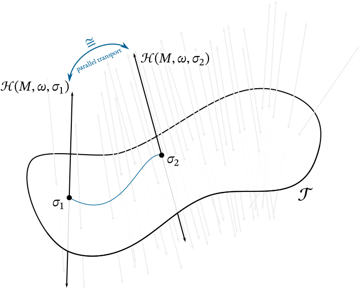
The other way to think about this was pioneered by Axelrod, della Pietra, Witten, and Hitchin. Suppose that you have a collection of polarizations that can be parametrized by a manifold $\mathcal{T}$. For each point $\sigma\in \mathcal{T}$, we have a polarization $P_\sigma$ in $TM$, and we can get the quantization $\mathcal{H}_\sigma$ with respect to this polarization. If the collection of polarizations is good enough, we hope that these quantizations can be put together into a vector bundle $\mathcal{H}$ over $\mathcal{T}$, such that $\mathcal{H}_\sigma$ is the fiber above $\sigma\in \mathcal{T}$.

If we have two polarizations represented by $\sigma_0$, $\sigma_1$, we can take a path $\sigma(t)$ in parameter space connecting them, and if we had a connection on this vector bundle, then parallel transport along $\sigma(t)$ would identify the fibers $\mathcal{H}_{\sigma_0}$ and $\mathcal{H}_{\sigma_1}$. However, this should be independent from the choice of the path, so the connection should be flat. Or almost. Now we play the “ah but quantum mechanics is in the projectivization of the Hilbert space!” card so it suffices to have a connection that is projectively flat. This is called a Hitchin connection.

Neither of these approaches has been proved in general, only in a few specific cases.

As a mathematical theory, geometric quantization has been steadily developed since its introduction in the late 60’s, and since then it has lost almost all of its intentions of becoming an useful theory for physics. My biggest gripe with it is the complete loss of focus on the observables: it focuses almost entirely on the construction of Hilbert space, and the quantization of observables is forgotten, which is ridiculous because that was the initial motivation for all the geometric constructions! The Hilbert space is the least important part of a quantum theory: there’s ways to do quantum mechanics without a Hilbert space, and interacting quantum field theory doesn’t even have a well-defined underlying Hilbert space of states. Quantum mechanics is a theory about observables, not states.

Oh no, I’m angry about geometric quantization again.

The gory details

First, we want to show that our first correction of the naive quantization rule breaks the commutations relations. The quantization rule is

\[f\mapsto \hat{f} = -i\hslash X_f + f.\]

So take $f, g\in C^\infty(M)$. We have

\[\begin{aligned} ~[\widehat{f},\widehat{g}] &= [-i\hslash X_f + f, -i\hslash X_g + g]\\ &= -\hslash^2[X_f,X_g] -i\hslash([f,X_g] + [X_f,g])\end{aligned}\]

The commutator of a vector field $X$ an a function $g$ acts on a function $\psi$ as

\[\psi = X[g\psi] - gX[\psi] = gX[\psi] + X[g]\psi - gX[\psi] = X[g]\psi,\]

and therefore we write

\[[X,g]= X[g].\]

With this, the commutator of $\hat{f}$ and $\hat{g}$ becomes

\[\begin{aligned} ~[\widehat{f},\widehat{g}] &= \hslash^2X_{\left\{f,g\right\}} -i\hslash(X_f[g] - X_g[f])\\ &= \hslash^2X_{\left\{f,g\right\}} -i\hslash(\left\{g,f\right\} - \left\{f,g\right\})\\ &= \hslash^2X_{\left\{f,g\right\}} +2i\hslash\left\{f,g\right\}\\ &= i\hslash\left(-i\hslash X_{\left\{f,g\right\}} +\left\{f,g\right\}\right) +i\hslash\left\{f,g\right\}\\ &= i\hslash(\widehat{\left\{f,g\right\}} + \left\{f,g\right\}).\end{aligned}\]

So indeed, we have a leftover term.

Now We want to show that once we choose a gauge (i.e. a symplectic potential) $\theta$, the quantization rule

\[f\mapsto \hat{f} = -i\hslash X_f + f - \theta(X_f)\]

satisfies the canonical commutation relations. From the result above, we can skip a few steps, since the terms $f$ and $\theta(X_g)$ commute (because they’re just multiplication by scalars).

\[\begin{aligned} ~[\widehat{f},\widehat{g}] & = [-i\hslash X_f + f - \theta(X_f),-i\hslash X_g + g - \theta(X_g)]\\ &= \hslash^2X_{\left\{f,g\right\}} +2i\hslash\left\{f,g\right\} +i\hslash([X_f,\theta(X_g)] +[\theta(X_f),X_g])\\ &= \hslash^2X_{\left\{f,g\right\}} +2i\hslash\left\{f,g\right\} +i\hslash(X_f[\theta(X_g)] -X_g[\theta(X_f)]).\end{aligned}\]

Now we use the fact that for any $1$-form $\alpha$ and vector fields $X,Y$,

\[\mathrm{d}{\alpha}(X,Y) = X[\alpha(Y)] - Y[\alpha(X)] - \alpha([X,Y]),\]

so that the rightmost term is

\[\begin{aligned} X_f[\theta(X_g)] -X_g[\theta(X_f)] &= \mathrm{d}{\theta}(X_f,X_g) + \theta([X_f,X_g])\\ &= -\omega(X_f,X_g) -\theta(X_{\left\{f,g\right\}})\\ &= -\left\{f,g\right\} - \theta(X_{\left\{f,g\right\}}).\end{aligned}\]

Putting everything back together, we get

\[\begin{aligned} ~[\widehat{f},\widehat{g}] &= \hslash^2X_{\left\{f,g\right\}} +2i\hslash\left\{f,g\right\} -i\hslash\left\{f,g\right\} - i\hslash\theta[X_{\left\{f,g\right\}}]\\ &=i\hslash\left( -i\hslash X_{\left\{f,g\right\}} +\left\{f,g\right\} - \theta[X_{\left\{f,g\right\}}]\right)\\ &=i\hslash\widehat{\left\{f,g\right\}}.\end{aligned}\]

References

• Segal, I.E., Quantization of Nonlinear Systems. Journal of Mathematical Physics 1, 468 (1960).

• Ali, S. T. and Engliš, M. Quantization Methods: A Guide for Physicists and Analysts. Rev. Math. Phys. 17, 391–490 (2005).

• Puta, M. Hamiltonian Mechanical Systems and Geometric Quantization. (Springer Netherlands, 1993).

• Woodhouse, N. M. J. Geometric Quantization. (Clarendon Press ; Oxford University Press, 1992).

• McDuff, D. and Salamon, D. Introduction to Symplectic Topology. (Oxford University Press, 2017).