A few months ago I was writing notes about things for my PhD and I had a lot of fun making the figures for it.
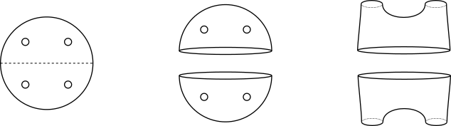
This one depicts slicing a sphere with two holes in half to obtain two things that are topologically equivalent to a pair-of-pants. I thought, huh this this a lot of fun let’s make more pretty pictures unrelated to my PhD. I’m reasonably good at basic math,[citation needed] I’m not terrible at programming,[citation needed] and I like geometric art so I can put those together and make
G E N E R A T I V E A R T
which means having a computer make the pretty pictures for me so I don’t need the amazing manual skills that other artists have and I don’t because I don’t have the patience to learn new things.
I think this is a good a time as any to plug my Instagram account where I post these and other pieces of generative art.
Here’s a few highlights of my favorites and the math behind them.
Rhumb line
A rhumb line is a curve of constant heading on a sphere. If you’re flying on a plane and you keep your compass in the same position, you’ll trace a rhumb line. A fun thing about them is that they wrap infinitely many times around the poles, in finite time!
Let’s parametrize the sphere with latitude $\lambda\in [-\pi/2,\pi/2]$ and longitude $\varphi\in [0,2\pi)$, so that a point on the unit sphere has coordinates $x, y , z$ given by
\[\begin{aligned} x &= \cos\lambda\cos\varphi,\\ y &= \cos\lambda\sin\varphi,\\ z &= \sin\lambda. \end{aligned}\]We want to find a curve $\gamma(t)$ whose tangent vector forms a constant angle $\beta$ with the unit vector in the $\lambda$ direction. At the point with coordinates $(\lambda,\varphi)$, tangent space is generated by the orthonormal vectors $\hat{\lambda},\hat{\varphi}$, given by
\[\begin{aligned} \hat{\lambda} &= -\sin\lambda\cos\varphi\hat{x} -\sin\lambda\sin\varphi \hat{y} +\cos\lambda\hat{z}\\ \hat{\varphi} &= -\sin\varphi\hat{x} + \cos\varphi\hat{y}. \end{aligned}\]So we want the tangent vector $\dot{\gamma}$ to be
\[\dot{\gamma} = \cos\beta\hat{\lambda} + \sin\beta\hat{\varphi}.\]If we write $\gamma(t)$ as a function of the latitute and longitude $\lambda(t),\varphi(t)$, i.e. very explicitly
\[\gamma(t) = x(\lambda(t),\varphi(t))\hat{x}+y(\lambda(t),\varphi(t))\hat{y} + z(\lambda(t),\varphi(t)\hat{z},\]then from the chain rule and the expressions for $\hat{\lambda},\hat{\varphi}$ we obtain
\[\dot{\gamma} = \dot{\lambda}\hat{\lambda} + \cos\lambda\dot{\varphi}\hat{\varphi}.\]Comparing with our desired $\dot\gamma = \cos\beta\hat{\lambda} + \sin\beta\hat\varphi$, we get a first-order ODE on $\lambda(t),\varphi(t)$:
\[\begin{aligned} \dot{\lambda} &= \cos\beta,\\ \dot\varphi &= \frac{\sin\beta}{\cos\lambda}, \end{aligned}\]which has a solution
\[\begin{aligned} \lambda(t) &= \lambda_0 + t\cos\beta\\ \varphi(t) &= \varphi_0 + \tan\beta\ln\left(\frac{\sec\lambda(t)-\tan\lambda(t)}{\sec\lambda_0 - \tan\lambda_0}\right). \end{aligned}\]A nice side-effect of this solution is that this is a constant speed parametrization of the curve. In fact, the speed is always $1$, so the parameter $t$ is also the arc-length of the curve. So $\varphi$ goes berserk and shoots off to infinity as you reach $\lambda = \pm \pi/2$, which means that the rhumb line wraps around the pole infinitely many times, but it remains finite in length!
The magnetic “pendulum”
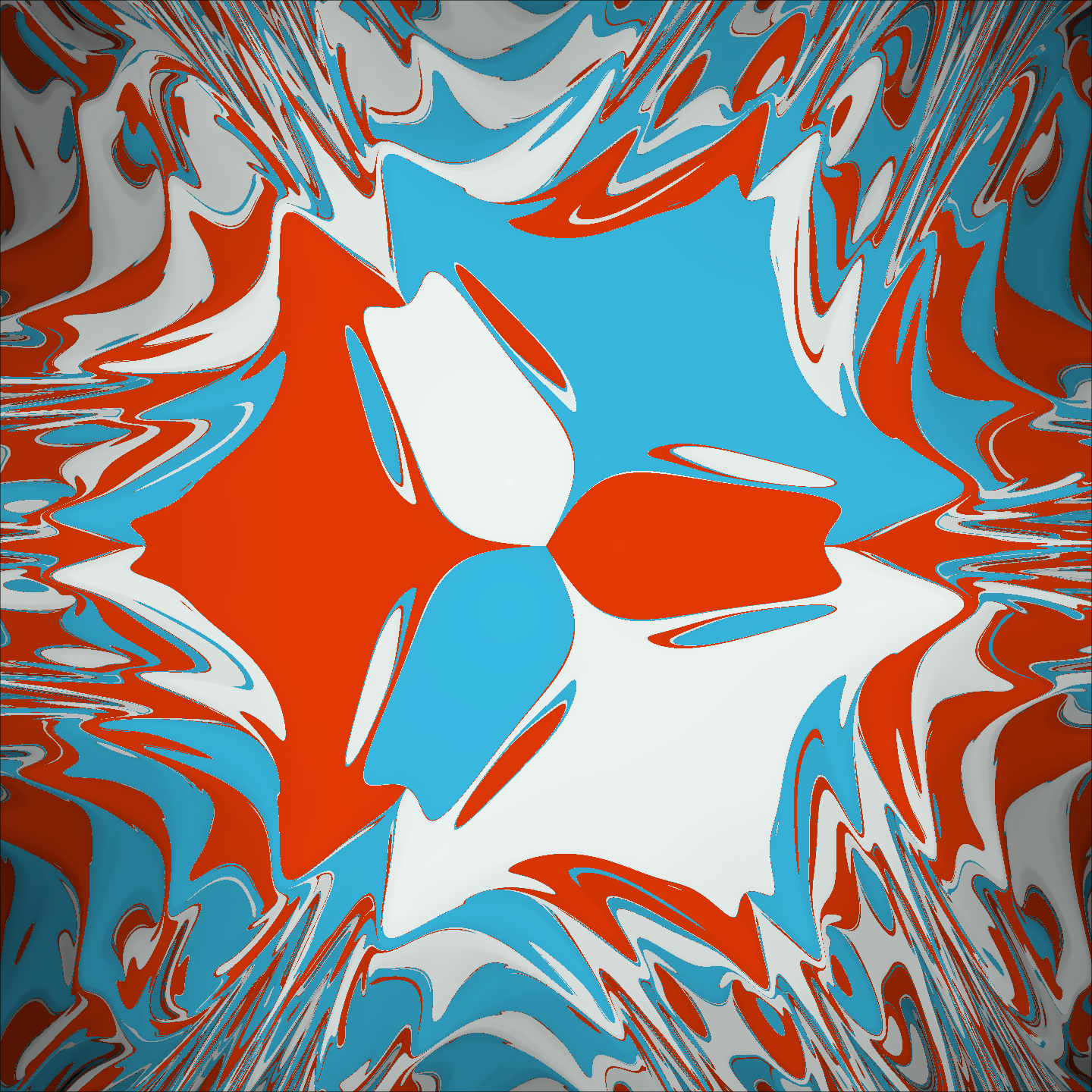
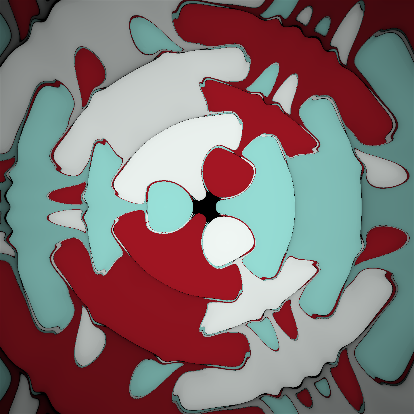
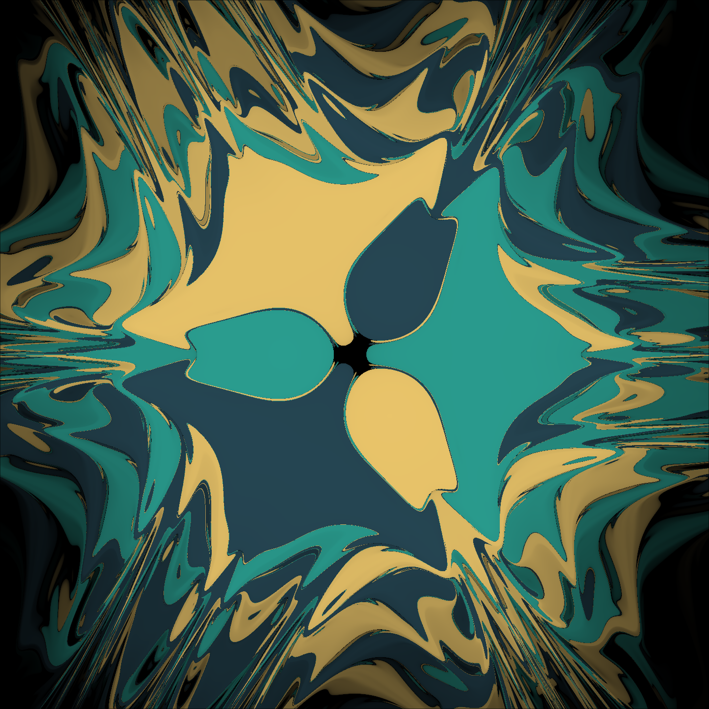
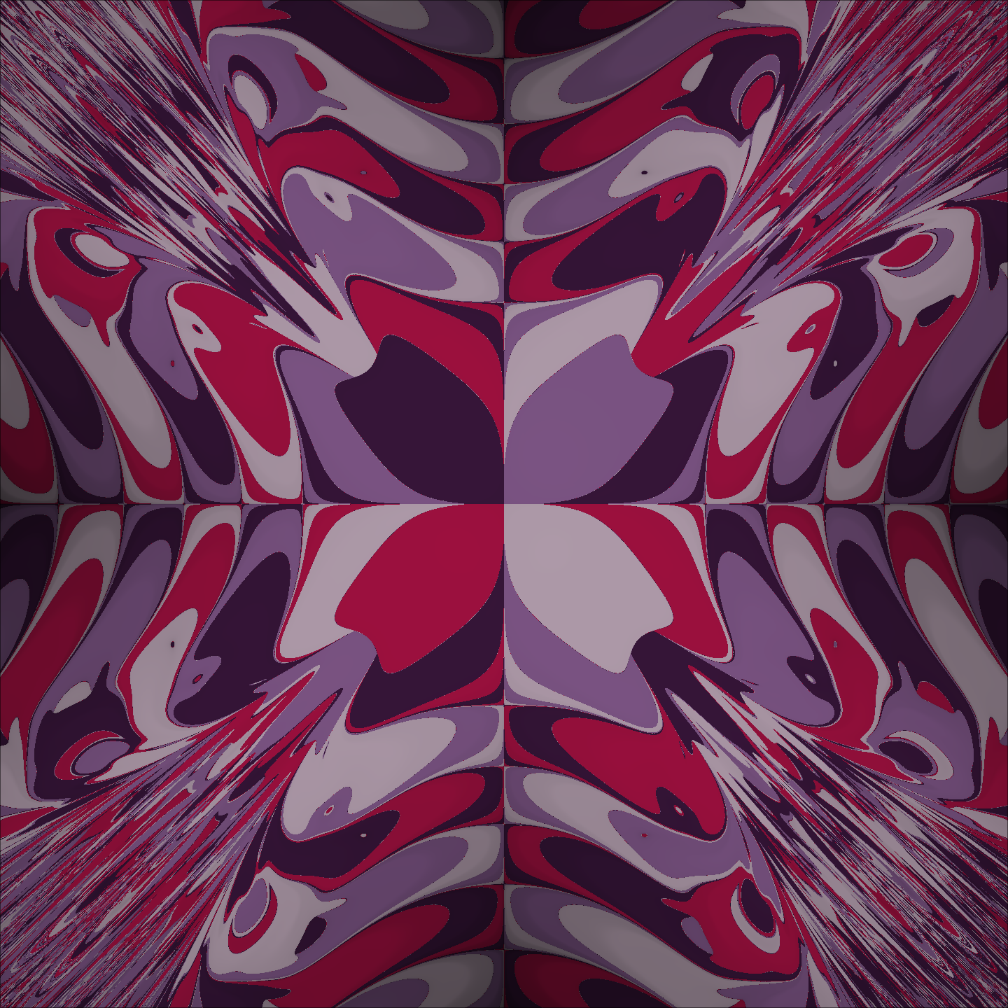
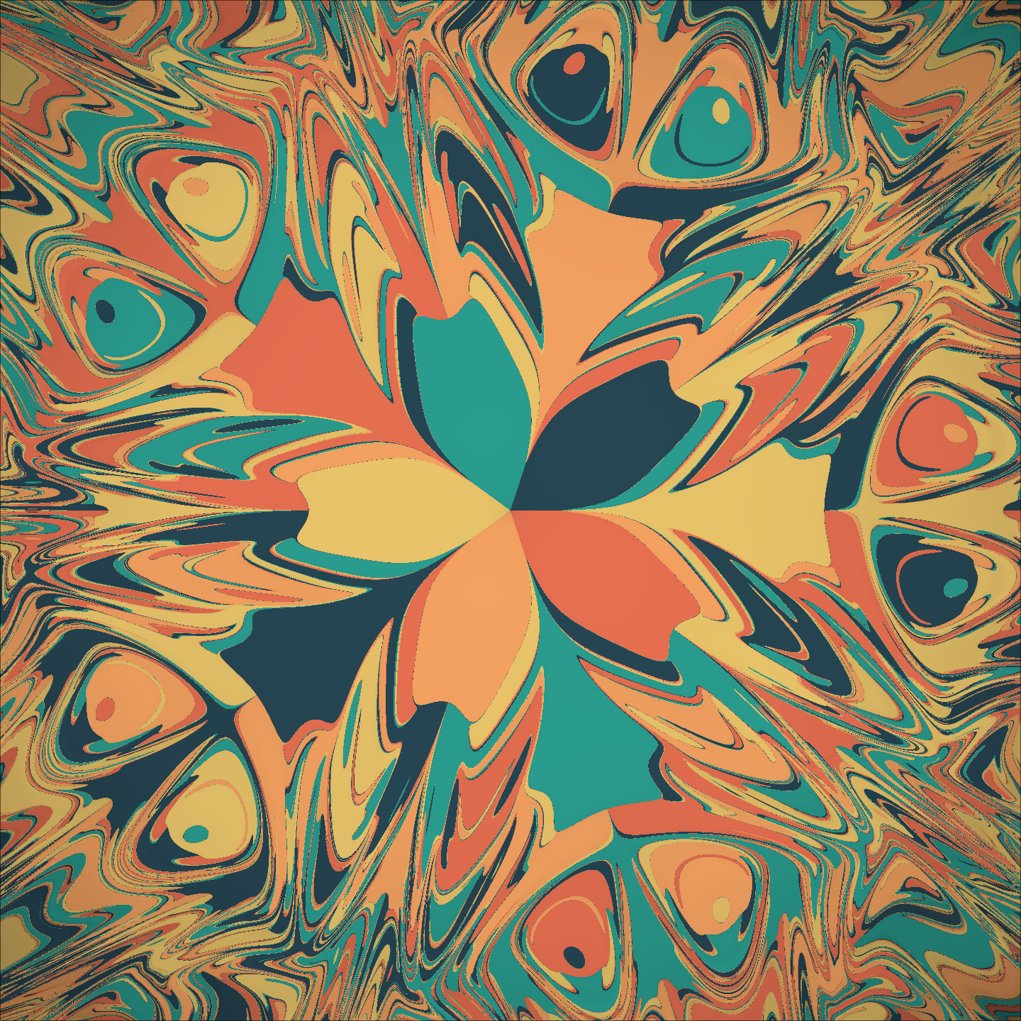
This is a typical example of a chaotic system. Consider a spherical pendulum with a magnetic bob. Nearby, on a plane below the lowest equilibrium point, there are three (or more) magnets. After releasing the bob, gravity and the three magnets start pushing it around, until it eventually settles due to friction. If the magnets are strong enough, the pendulum will settle above one of them.
If we assume that the pendulum is very long or that the oscillations are small, then we can approximate the pendulum as a two-dimensional harmonic oscillator. In this case, if $x$ is the position of the pendulum and $x_i$ are the positions of the magnets with “magnetic charges” $q_i$, then the total force acting on the bob is
\[F = -kx - b\dot x+ \sum_i \frac{q_i}{(\|x-x_i\|^2 + h^2)^{5/2}}(x-x_i),\]where $k$ is a parameter representing gravity, $h$ is the distance from the plane where the magnets are to the minimum height of the pendulum, and $b$ is a parameter that controls viscous drag. We generate this image as follows: For every pixel, integrate the equations of motion with starting point at that pixel, from rest. Eventually, the system settles over one of the magnets. We color the pixel according to the magnet where it ended up. As an aside, I used a GLSL shader to generate these images, because well, that’s a lot of iterations.
The Hopf bundle
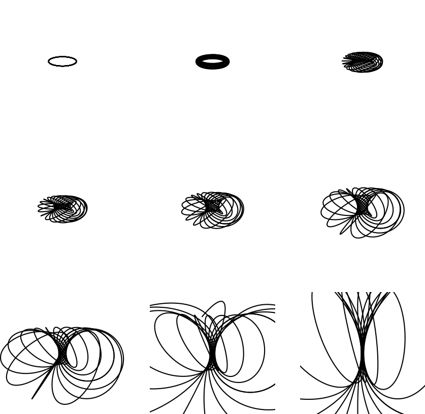
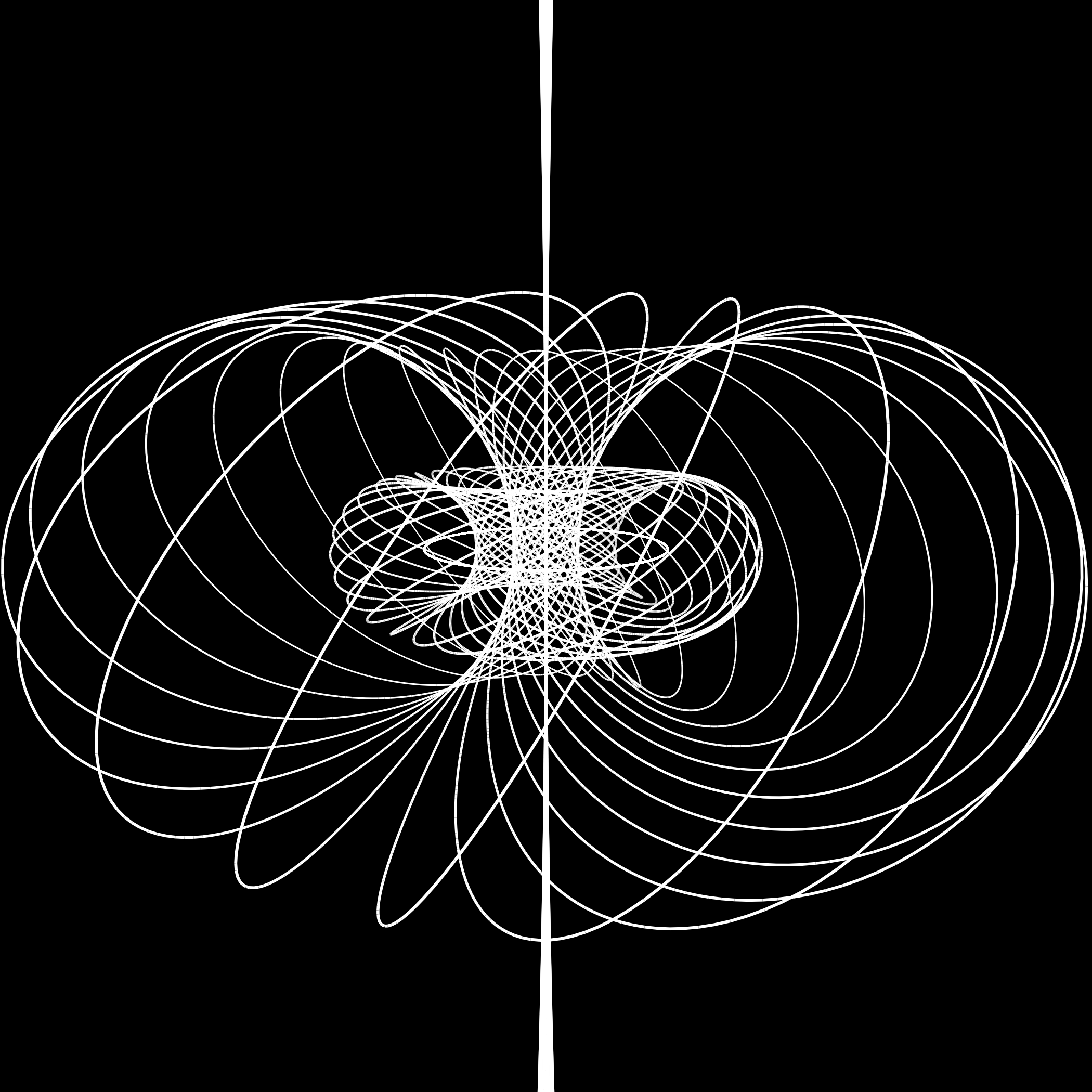
I still don’t know how to make something pretty with this aside from showing some of the fibers, but the mathematics is pretty nice. Colors would be nice, but I had some issues with rendering that made colors impossible.
Consider the 3-sphere $S^3$ as a subset of $\mathbb{C}^2$: \(S^3 = \{(z_1,z_2)\in\mathbb{C}^2:|z_1|^2 + |z_2|^2 = 1\}.\) From the defining equation $|z_1|^2 + |z_2|^2 = 1$, we can choose an angle $\theta\in[0,\pi]$ such that $|z_1| = \cos(\theta/2)$ and $|z_2| = \sin(\theta/2)$. Then we can write
\[\begin{aligned} z_1 &= \cos(\theta/2)e^{i\xi_1}\\ z_2 &= \sin(\theta/2)e^{i\xi_2} \end{aligned}\]for some unique $\xi_1$, $\xi_2\in[0,2\pi)$. If we just look at the parameters $\theta,\xi_1$ and $\xi_2$, it seems that we have a line segment and two circles. However, when $\theta = 0$ and $\theta = \pi$, the points “collapse” in a way, since either $z_1$ or $z_2$ are fixed at zero. That makes one of the parameters $\xi$ irrelevant at those points.
Compare this with the parametrization of the $2$-sphere $S^2$ with spherical coordinates $\theta$ and $\varphi$, where $\theta$ is the zenithal coordinate and $\varphi$ is the azimuthal coordinate. When $\theta = 0$ or $\theta = \pi$, then $\varphi$ becomes irrelevant because a horizontal slice of the sphere collapses from a circle to a point.
This kinda suggests that we can intuitively think of $S^3$ as $S^2$ with a bunch of circles attached to every point. Let’s make it precise: Define a map $f:S^3\to S^2$, where $f(z_1,z_2)$ is the point with zenithal coordinate $\theta$ defined as above, and with azimuthal coordinate $\varphi = \xi_2 - \xi_1$. We can make this very explicit. From the definition above, we have that
\[\begin{aligned} \sin(\theta) &= 2|z_1 z_2|,\\ \cos(\theta) &= |z_1|^2 + |z_2|^2,\\ \sin(\varphi) &= \left|\frac{z_1}{z_2}\right|\operatorname{Im}\left(\frac{z_2}{z_1}\right),\\ \cos(\varphi) &= \left|\frac{z_1}{z_2}\right|\operatorname{Re}\left(\frac{z_2}{z_1}\right), \end{aligned}\]and so $f(z_1,z_2)\in S^2$ is the point with coordinates $(x,y,z)$ given by
\[\begin{aligned} x &= 2|z_1|^2\operatorname{Re}\left(\frac{z_2}{z_1}\right),\\ y &= 2|z_1|^2\operatorname{Im}\left(\frac{z_2}{z_1}\right),\\ z &= |z_1|^2 + |z_2|^2. \end{aligned}\]The map $f:S^3\to S^2$ is surjective, and it is invariant under the $S^1$ action $(z_1,z_2)\cdot e^{i\lambda} = (e^{i\lambda}z_2,e^{i\lambda}z_2)$. In fact, if we fix a point on the fiber, then every other point on it can be reached by this action in a unique way. We say that the action is transitive and free on the fibers. Therefore, the fibers of $f$ are circles, and we can write $S^3$ as the union of all these circle fibers over the sphere.
The next problem is trying to visualize the fibers. This is a big issue because our monkey brain only understands figures that can be embedded in three-dimensional euclidean space. So now our task is to “flatten out” $S^3$ onto $\mathbb{R}^3$, very much in the same way that we would want to flatten out the sphere (like the surface of Earth) onto the plane (as if to make a map). I guess there’s many different ways to do this, like there are many different spherical projections for cartography, but we are going to stick with the easiest one: Stereographic projection. I won’t go into details, but the wikipedia page is a good place to start. We have an easy formula for this projection $P:S^3\to \mathbb{R}^3$. If we write a point on $S^3$ as $(\mathbf{x},h)$ with $\mathbf{x}\in \mathbb{R}^3$, then
\[P(\mathbf{x},h) = \frac{1}{1-h}\mathbf{x}.\]So now the visualization goes as follows: Choose a point on the sphere $S^2$ with coordinates $(\theta,\varphi)$. This point does not determine a unique element of $S^3$, but an entire circle. We can parametrize the entire circle by finding a single point on the fiber, and then acting with the circle action:
\[f^{-1}(\theta,\varphi) = \{(\cos(\theta/2)e^{i(\lambda+\varphi)},\sin(\theta/2)e^{i\lambda}):\lambda\in[0,2\pi) \}.\]Now we project the points to $\mathbb{R}^3$ with the stereographic projection. In the end, we obtain a map parametrizing the fibers after projecting them:
\[\mathrm{fiber}(\theta,\varphi,\lambda) = \frac{1}{1-\sin(\theta/2)\sin(\lambda)}(\cos(\theta/2)\cos(\lambda+\varphi),\cos(\theta/2)\sin(\lambda+\varphi),\sin(\theta/2)\cos(\lambda)).\]The Hopf fibration is a prime example of a principal bundle, and it shows up here and there in mathematics and physics. Most notably, in the quantization of the Dirac monopole, the wavefunctions become sections of the associated bundle to the Hopf bundle via some representation of $U(1)$. You can see my notes on connections on principal bundles for explanations of some of these terms, but I plan to write something more detailed on the Hopf bundle and the Dirac monopole sometime in the future.