Get the pdf version of this post here.

This time we’re going to be more concrete. The general theory of many-particle states can be quite tricky and unintuitive, so it’s better to start everything with the simplest example: a 2-state system.

Last time in Homotopico, we derived the Hilbert spaces that correspond to multiple identical particles. If a single particle is represented by the Hilbert space $ \mathcal{H}$, then there are two kinds of indistiguishable $k$-particle spaces: the bosonic space $ \mathcal{S}^k \mathcal{H}$ and the fermionic space $\Lambda^k \mathcal{H}$. These spaces are defined in terms of the permutation operators $P_\sigma$ (in the previous post I called them $T_\sigma$), which are the natural representation of the permutation group $ \mathfrak{S}_k$ on $\otimes^k \mathcal{H}$: for each $\sigma\in \mathfrak{S}_k$, define

\[P_\sigma{\vert \psi_1\dots\psi_k \rangle}={\vert \psi_{\sigma(1)}\dots\psi_{\sigma(k)} \rangle}.\]

The bosonic space is composed of vectors that are permutation invariant,

\[\mathcal{S}^k \mathcal{H} = {\left\{ {\vert \Psi \rangle} \in \otimes^k \mathcal{H}~:~P_\sigma{\vert \Psi \rangle}={\vert \Psi \rangle}\quad \forall\sigma\in \mathfrak{S}_k\right\}},\]

while the fermionic space is composed of vectors that are reversed under odd permutations, i.e.

\[\Lambda^k \mathcal{H} = {\left\{ {\vert \Psi \rangle} \in \otimes^k \mathcal{H}~:~P_\sigma{\vert \Psi \rangle}=\operatorname{sgn}(\sigma){\vert \Psi \rangle}\quad \forall\sigma\in \mathfrak{S}_k\right\}}.\]

It can be checked that these are indeed Hilbert spaces (we won’t do that here). What we will do now is constructing state spaces with an arbitrary number of particles, instead of a fixed number of particles. Here, we will first focus on a 2-state system, for example polarization of photons or spin-$\frac{1}{2}$.

Two states one particle

When we talk about a system with $2$ states, we really mean that the Hilbert space $ \mathcal{H}$ is of (complex) dimension $2$. This tells us that we can find a basis $\left\{ {\vert a \rangle},{\vert b \rangle}\right\}$, such that ${\left\langle a \middle\vert a\right\rangle}={\left\langle b \middle\vert b\right\rangle}=1$ and ${\left\langle a \middle\vert b\right\rangle}=0$. In the case of spin-$\frac{1}{2}$ systems, ${\vert a \rangle},{\vert b \rangle}$ are normalized eigenstates of some spin operator, often $\hat{S}_z$. In the case of photon polarization, ${\vert a \rangle},{\vert b \rangle}$ represent states of pure horizontal or vertical polarization with respect to some axis. What the kets ${\vert a \rangle}$ and ${\vert b \rangle}$ actually stand for (physically speaking) is irrelevant for our discussion. What is important is that we have an orthonormal basis that consists of $2$ vectors, which means that any (one-particle) state in $ \mathcal{H}$ can be written as

\[{\vert \psi \rangle} = \alpha{\vert a \rangle} + \beta{\vert b \rangle},\]

with $\alpha,\beta\in {\mathbb{C}}$.

2-particle states

We now stick two of these one-particle spaces together via the tensor product. Recall that $ \mathcal{H}\otimes \mathcal{H}$ is the vector space of linear combinations of elements of the form ${\vert \psi_1\psi_2 \rangle}:={\vert \psi_1 \rangle}\otimes{\vert \psi_2 \rangle}$ with ${\vert \psi_1 \rangle},{\vert \psi_2 \rangle}\in \mathcal{H}$. Since we have a basis ${\vert a \rangle},{\vert b \rangle}$ of $ \mathcal{H}$, we can write

\[\begin{aligned} {\vert \psi_1 \rangle} &= \alpha_1{\vert a \rangle} + \beta_1{\vert b \rangle}\\ {\vert \psi_2 \rangle} &= \alpha_2{\vert a \rangle} + \beta_2{\vert b \rangle}, \end{aligned}\]

so that

\[{\vert \psi_1\psi_2 \rangle} = (\alpha_1{\vert a \rangle} + \beta_1{\vert b \rangle})\otimes(\alpha_2{\vert a \rangle} + \beta_2{\vert b \rangle}) = \alpha_1\alpha_2{\vert aa \rangle} + \alpha_1\beta_2{\vert ab \rangle} + \beta_1\alpha_2{\vert ba \rangle} + \beta_1\beta_2{\vert bb \rangle}.\]

This means that, in general, any element of $ \mathcal{H}\otimes \mathcal{H}$ can be written as a linear combination of ${\vert aa \rangle},{\vert ab \rangle},{\vert ba \rangle},{\vert bb \rangle}$. However, not every element of $ \mathcal{H}\otimes \mathcal{H}$ can be written as ${\vert \psi_1\psi_2 \rangle}$ for some ${\vert \psi_1 \rangle},{\vert \psi_2 \rangle}\in \mathcal{H}$. The elements that can be written in this way are called product states.

If we define the inner product in $ \mathcal{H}$ as

\[{\left\langle \psi_1\otimes \psi_2 \middle\vert \phi_1\otimes\phi_2\right\rangle}:={\left\langle \psi_1 \middle\vert \phi_1\right\rangle}{\left\langle \psi_2 \middle\vert \phi_2\right\rangle},\]

it can be easily shown that $\left\{ {\vert aa \rangle},{\vert ab \rangle},{\vert ba \rangle},{\vert bb \rangle} \right\}$ forms an orthonormal basis of $ \mathcal{H}\otimes \mathcal{H}$.

We interpret the state ${\vert \psi_1\psi_2 \rangle}$ as saying “particle 1 is in state ${\vert \psi_1 \rangle}$ and particle 2 is in state ${\vert \psi_2 \rangle}$”. Since in general ${\vert \psi_1\psi_2 \rangle}\neq{\vert \psi_2\psi_1 \rangle}$, under this interpretation our particles are distinguishable. Indeed, that’s why it even makes sense to speak of particle 1 and particle 2.

Introducing indistinguishability

In the previous post, we explained that the spaces of indistinguishable particles are those in which the permutation transformation $P: \mathcal{H}\otimes \mathcal{H}\to \mathcal{H}\otimes \mathcal{H}$, given by

\(P{\vert \psi_1\psi_2 \rangle} := {\vert \psi_2\psi_1 \rangle},\) and extended everywhere by linearity, is an absolute symmetry. Equivalently, a state ${\vert \Psi \rangle}\in \mathcal{H}\otimes \mathcal{H}$ (not necessarily a product state!) represents indistinguishable particles if and only if \(P{\vert \Psi \rangle} = \pm{\vert \Psi \rangle}.\) The bosonic states are the ones for which $P{\vert \Psi \rangle}={\vert \Psi \rangle}$, and the fermionic states are the ones for which $P{\vert \Psi \rangle} = -{\vert \Psi \rangle}$. In the previous post we showed that given a product state ${\vert \Psi \rangle}= {\vert \psi_1\psi_2 \rangle}$, the state

\[\frac{1}{2}\left({\vert \psi_1\psi_2 \rangle}+{\vert \psi_2\psi_1 \rangle}\right)\]

is a bosonic state, while

\[\frac{1}{2}\left({\vert \psi_1\psi_2 \rangle}-{\vert \psi_2\psi_1 \rangle}\right)\]

is a fermionic state, and neither is necessarily normalized. Indeed, all the bosonic and fermionic 2-particle states are expressed as linear combinations of elements of that form! To see this, consider an arbitrary state ${\vert \Psi \rangle}$. We can write it in terms of the basis as

\[{\vert \Psi \rangle} = \alpha_{11}{\vert aa \rangle} + \alpha_{12}{\vert ab \rangle} + \alpha_{21}{\vert ba \rangle} + \alpha_{22}{\vert bb \rangle},\]

where $\alpha_{11},\dots,\alpha_{22}\in {\mathbb{C}}$ are complex numbers. Now we apply $P$:

\[\begin{aligned} P{\vert \Psi \rangle} &= \alpha_{11}P{\vert aa \rangle} + \alpha_{12}P{\vert ab \rangle} + \alpha_{21}P{\vert ba \rangle} + \alpha_{22}P{\vert bb \rangle}\\ &= \alpha_{11}{\vert aa \rangle} + \alpha_{12}{\vert ba \rangle} + \alpha_{21}{\vert ab \rangle} + \alpha_{22}{\vert bb \rangle}. \end{aligned}\]

If $P{\vert \Psi \rangle}=\pm{\vert \Psi \rangle}$, this tells us that

\[\begin{aligned} \alpha_{11}&=\pm\alpha_{11}\\ \alpha_{12}&=\pm\alpha_{21}\\ \alpha_{22}&=\pm\alpha_{22}. \end{aligned}\]

Note that if $P{\vert \Psi \rangle}=-{\vert \Psi \rangle}$ (i.e. ${\vert \Psi \rangle}$ is fermionic), then $\alpha_{11}=-\alpha_{11}$, which means that $\alpha_{11}=0$, and similarly $\alpha_{22}=0$. Substituting back in ${\vert \Psi \rangle}$ for the general case, we obtain:

\[\begin{aligned} {\vert \Psi \rangle} &= \alpha_{11}{\vert aa \rangle} + \alpha_{12}{\vert ab \rangle} + \alpha_{21}{\vert ba \rangle} + \alpha_{22}{\vert bb \rangle}\\ &= \alpha_{11}{\vert aa \rangle} + \alpha_{12}{\vert ab \rangle} \pm \alpha_{12}{\vert ba \rangle} + \alpha_{22}{\vert bb \rangle}\\ &=\alpha_{11}{\vert aa \rangle} + \alpha_{12}\left({\vert ab \rangle} \pm {\vert ba \rangle}\right) + \alpha_{22}{\vert bb \rangle}\\ &=\frac{\alpha_{11}}{2}({\vert aa \rangle}\pm {\vert aa \rangle}) + \frac{2\alpha_{12}}{2}\left({\vert ab \rangle} \pm {\vert ba \rangle}\right) + \frac{\alpha_{22}}{2}({\vert bb \rangle}\pm{\vert bb \rangle}),\qquad (\star) \end{aligned}\]

and therefore indeed ${\vert \Psi \rangle}$ is a linear combination of elements of the form

\[\frac{1}{2}({\vert \psi_1\psi_2 \rangle}\pm{\vert \psi_2\psi_1 \rangle}).\]

In particular, we can find bases for the boson and fermion 2-particle states. From equation $(\star)$ we see that a basis for the boson space is given by

\[{\vert aa \rangle},\quad \frac{1}{2}({\vert ab \rangle}+{\vert ba \rangle}),\quad{\vert bb \rangle}.\]

and so the boson space has dimension $3$. We can now orthonormalize this basis, to obtain a (you guessed it), orthonormal basis. It turns out that these three elements are already orthogonal, and ${\vert aa \rangle},{\vert bb \rangle}$ are already normalized (why?) so we only need to normalize the remaining one. This means that we have to calculate its norm:

\[\begin{aligned} \|({\vert ab \rangle}+{\vert ba \rangle})\|^2 & ={\left\langle ab+ba \middle\vert ab+ba\right\rangle}\\ &=\left({\left\langle ab \middle\vert ab\right\rangle} + {\left\langle ab \middle\vert ba\right\rangle} + {\left\langle ba \middle\vert ab\right\rangle} +{\left\langle ba \middle\vert ba\right\rangle}\right)\\ &=\left({\left\langle a \middle\vert a\right\rangle}{\left\langle b \middle\vert b\right\rangle} + {\left\langle a \middle\vert b\right\rangle}{\left\langle b \middle\vert a\right\rangle} + {\left\langle b \middle\vert a\right\rangle}{\left\langle a \middle\vert b\right\rangle} +{\left\langle b \middle\vert b\right\rangle}{\left\langle a \middle\vert a\right\rangle}\right)\\ &=(1+0+0+1)\\ &=2, \end{aligned}\]

And this tells us that the normalized state is

\(\frac{1}{\sqrt{2}}({\vert ab \rangle}+{\vert ba \rangle}).\) We have now obtained an orthonormal basis for the boson space, which we call the occupation number basis. We define it as

\[\begin{aligned} {\vert 2,0 \rangle} &:= {\vert aa \rangle}\\ {\vert 1,1 \rangle} &:= \frac{1}{\sqrt{2}}({\vert ab \rangle}+{\vert ba \rangle})\\ {\vert 0,2 \rangle} &:= {\vert bb \rangle}. \end{aligned}\]

We interpret ${\vert 2,0 \rangle}$ as a state with two particles in state ${\vert a \rangle}$ and no particles in state ${\vert b \rangle}$, ${\vert 1,1 \rangle}$ as a state with one particle in each state${\vert a \rangle},{\vert b \rangle}$, and ${\vert 0,2 \rangle}$ as a state with no particles in state ${\vert a \rangle}$ and two particles in state ${\vert b \rangle}$ (see image below).

Similarly, from equation $(\star)$ for fermions, we see that a basis is given by the single element

\[{\vert ab \rangle} = \frac{1}{2}({\vert ab \rangle}-{\vert ba \rangle}).\]

Therefore we conclude that the fermion space is $1$-dimensional. We can normalize this state to obtain the occupation number basis for fermions (which in this case is a single, lonely state):

\[{\vert 1,1 \rangle} := \frac{1}{\sqrt{2}}({\vert ab \rangle}-{\vert ba \rangle}).\]

Note that there are no other independent states, and unlike the bosonic case, we don’t have states that represent two particle in the same state. For fermions, no two particles are ever in the same state: this is called Pauli’s exclusion principle.

3-particle states

Instead of jumping to the general $n$-particle case, we will consider the 3-particle states. Here, the permutations are much more complicated, and so a thorough understanding of this case will give us a good intuition to work on the general case.

Our “distinguishable” 3-particle space is $\otimes^3 \mathcal{H}= \mathcal{H}\otimes \mathcal{H}\otimes \mathcal{H}$, which is the vector space of linear combinations of elements of the form ${\vert \psi_1\psi_2\psi_3 \rangle}={\vert \psi_1 \rangle}\otimes{\vert \psi_2 \rangle}\otimes{\vert \psi_3 \rangle}$ for ${\vert \psi_j \rangle}\in \mathcal{H}$. Following the exact same procedure as above, we can see that any element of $\otimes^3 \mathcal{H}$ can be expressed as

\[\begin{aligned} {\vert \Psi \rangle} &=\phantom{+} \alpha_{111}{\vert aaa \rangle} + \alpha_{112}{\vert aab \rangle} + \alpha_{121}{\vert aba \rangle} + \alpha_{122}{\vert abb \rangle}\\ &\phantom{=} + \alpha_{211}{\vert baa \rangle} + \alpha_{212}{\vert bab \rangle} + \alpha_{221}{\vert bba \rangle} +\alpha_{222}{\vert bbb \rangle}, \end{aligned}\]

for $\alpha_{ijk}\in {\mathbb{C}}$, and $i,j,k =1,2$.

Introducing indistinguishability

Here’s where things get tricky, since there are many more permutations. This means that we need to introduce a little bit more notation. Recall that a permutation of $k$ numbers is a function $\sigma$ that reorders the set $(1,2,\dots,k)$. For example, the function defined as $\sigma(1)=2$, $\sigma(2)=3$ and $\sigma(3)=1$ is a permutation of $(1,2,3)$. We may write it more concisely as $\sigma = (2,3,1)$, or in general, $\sigma = (\sigma(1),\dots,\sigma(k))$ for a permutation of $k$ numbers. The set of all permutations of $k$ numbers is denoted by $ \mathfrak{S}_k$. It can be shown that it is a group under composition, and that it has exactly $k!$ elements.

Now in the case of $3$ particles, we need to consider permutations of $3$ numbers. There are $3!=6$ such permutations, namely:

\[\begin{align*} (1,2,3) \quad (3,1,2) \quad (2,3,1) \\ (1,3,2) \quad (2,1,3) \quad (3,2,1) \end{align*}.\]

Let’s recall the natural action of $ \mathfrak{S}_3 $ on $\otimes^3 \mathcal{H}$. For each $\sigma\in \mathfrak{S}_3 $, define an operator $P_\sigma$ which acts on product states as

\[P_\sigma{\vert \psi_1\psi_2\psi_3 \rangle}={\vert \psi_{\sigma(1)}\psi_{\sigma(2)}\psi_{\sigma(3)} \rangle}.\]

This action is extended by linearity everywhere else (recall that not all elements are product states!). As a particular example, choose $\sigma = (3,1,2)$. So we have

\[P_\sigma{\vert \psi_1\psi_2\psi_3 \rangle}={\vert \psi_{3}\psi_{1}\psi_{2} \rangle}.\]

To be a bit more explicit, suppose ${\vert \Psi \rangle}= {\vert aba \rangle}-2{\vert bba \rangle}$. Then

\[P_\sigma{\vert \Psi \rangle}=P_\sigma{\vert aba \rangle}-2P_\sigma{\vert bba \rangle} = {\vert aab \rangle}-2{\vert abb \rangle}.\]

As before, in order to talk about indistinguishability, we need to restrict ourselves to a subspace of $\otimes^3 \mathcal{H}$ where the action of $ \mathfrak{S}_3$ is an absolute unitary symmetry. In the previous post we showed that the only way is if either

\(P_{\sigma}{\vert \Psi \rangle} = {\vert \Psi \rangle},\) which is the bosonic case, or if

\[P_{\sigma}{\vert \Psi \rangle} = (\operatorname{sgn}\sigma){\vert \Psi \rangle},\]

which is the fermionic case.

Same as before, we will find an explicit basis for these bosonic and fermionic subspaces. In this case the fermionic subspace is quite simple (perhaps too simple!), so we will start with it. Write ${\vert \Psi \rangle}$ again as

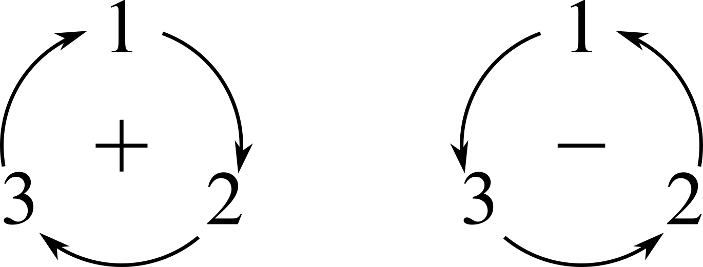
\[\begin{aligned} {\vert \Psi \rangle} &=\phantom{+} \alpha_{111}{\vert aaa \rangle} + \alpha_{112}{\vert aab \rangle} + \alpha_{121}{\vert aba \rangle} + \alpha_{122}{\vert abb \rangle}\\ &\phantom{=} + \alpha_{211}{\vert baa \rangle} + \alpha_{212}{\vert bab \rangle} + \alpha_{221}{\vert bba \rangle} +\alpha_{222}{\vert bbb \rangle}, \end{aligned},\]

and suppose that for all ${\sigma \in \mathfrak{S}_3}$, $P_\sigma{\vert \Psi \rangle}=(\operatorname{sgn}\sigma){\vert \Psi \rangle}$. The sign of a permutation of $3$ numbers is $1$ if it is a cyclic permutation of $(1,2,3)$, and $-1$ if it is a cyclic permutation of $(1,3,2)$, as in below.

.

For example, consider $\sigma = (1,3,2)$, for which $\operatorname{sgn}\sigma = -1$. Note that $\sigma$ switches the elements $2$ and $3$. Then we have

\[\begin{aligned} P_\sigma{\vert \Psi \rangle} &=\phantom{+} \alpha_{111}{\vert aaa \rangle} + \alpha_{112}{\vert aba \rangle} + \alpha_{121}{\vert aab \rangle} + \alpha_{122}{\vert abb \rangle}\\ &\phantom{=} + \alpha_{211}{\vert baa \rangle} + \alpha_{212}{\vert bba \rangle} + \alpha_{221}{\vert bab \rangle} +\alpha_{222}{\vert bbb \rangle}. \end{aligned}\]

However, we also need $P_\sigma{\vert \Psi \rangle}=-{\vert \Psi \rangle}$, so comparing above this implies that

\[\begin{aligned} \alpha_{111} &= -\alpha_{111} & \alpha_{122}&=-\alpha_{122} & \alpha_{211} &=-\alpha_{211} & \alpha_{222} &=-\alpha_{222}\\ & & \alpha_{112} &= -\alpha_{121} & \alpha_{212}&=-\alpha_{221}, & &\end{aligned}\]

and so $\alpha_{111}=\alpha_{122}=\alpha_{211}=\alpha_{222}=0$. Thus we write ${\vert \Psi \rangle}$ as

\[{\vert \Psi \rangle} = \alpha_{112}({\vert aab \rangle}-{\vert aba \rangle}) + \alpha_{212}({\vert bab \rangle}-{\vert bba \rangle}).\]

Now we consider $\sigma = (3,1,2)$, which is simply a cyclic permutation of $(1,2,3)$, and so $\operatorname{sgn}\sigma = 1$. We then have

\[P_{\sigma}{\vert \Psi \rangle} = \alpha_{112}({\vert baa \rangle}-{\vert aab \rangle}) + \alpha_{212}({\vert bba \rangle}-{\vert abb \rangle}) ={\vert \Psi \rangle},\]

and this again tells us that $\alpha_{112}=-\alpha_{112}$ and $\alpha_{212}=-\alpha_{212}$, so $\alpha_{112}=\alpha_{212}=0$. Therefore ${\vert \Psi \rangle}=0$ (!). This tells us that there are no 3-particle fermionic states if the single-particle space has only $2$ states! We see this again as a case of Pauli’s exclusion principle: there cannot be two particles in the same state, but we have $3$ particles that have to fit into only 2 states!

The bosonic case is a little bit more tedious, but let’s get to it. Again, expand $\Psi$ in terms of the basis vectors, and let’s impose $P_{\sigma}{\vert \Psi \rangle}={\vert \Psi \rangle}$ for all $\sigma\in \mathfrak{S}_3$. Let’s consider a small term, for example $\alpha_{112}{\vert aab \rangle}$. Applying $P_{\sigma}$, we obtain $\alpha_{112}{\vert baa \rangle}$, but the original coefficient that goes next to ${\vert baa \rangle}$ in the expansion of ${\vert \Psi \rangle}$ is $\alpha_{211}$, so this tells us that

\(\alpha_{112}=\alpha_{211}.\) Similarly, when we apply, for example $\sigma = (1,3,2)$ (as above!) we must have $\alpha_{112}=\alpha_{121}$. Therefore $\alpha_{112}=\alpha_{211}=\alpha_{121}$. Applying this exact same analysis, but to the term $\alpha_{221}{\vert bba \rangle}$, we obtain that $\alpha_{221}=\alpha_{212}=\alpha_{122}$, so that ${\vert \Psi \rangle}$ can be written as:

\[{\vert \Psi \rangle} = \alpha_{111}{\vert aaa \rangle} +\alpha_{112}({\vert aab \rangle}+{\vert aba \rangle}+{\vert baa \rangle}) + \alpha_{221}({\vert bba \rangle}+{\vert bab \rangle} + {\vert abb \rangle}) +\alpha_{222}{\vert bbb \rangle}.\]

This tells is that the subspace of bosonic states is generated by four vectors, namely:

\[{\vert aaa \rangle}; \qquad {\vert aab \rangle}+{\vert aba \rangle}+{\vert baa \rangle};\qquad {\vert bba \rangle}+{\vert bab \rangle} + {\vert abb \rangle}; \text{ and}\qquad {\vert bbb \rangle}.\]

Note that each of these elements is the sum over all the possible permutations of one of its terms. For example, the element ${\vert aab \rangle}+{\vert aba \rangle}+{\vert baa \rangle}$ is the sum over all permutations of ${\vert aab \rangle}$. In the case of ${\vert aaa \rangle}$ and ${\vert bbb \rangle}$, all permutations of them are themselves again! This is also true for the case of two particles: each of the basis elements of the bosonic space is the sum over all permutations of $2$ numbers (of which there are only two!) of the different basis elements.

Now, similarly as above, we normalize these four vectors (they are already orthogonal, why?), and obtain an orthonormal basis

\[\begin{aligned} {\vert 3,0 \rangle} &:= {\vert aaa \rangle},\\ {\vert 2,1 \rangle} &:= \frac{1}{\sqrt{3}}\left({\vert aab \rangle}+{\vert aba \rangle}+{\vert baa \rangle}\right),\\ {\vert 1,2 \rangle} &:= \frac{1}{\sqrt{3}}\left({\vert bba \rangle}+{\vert bab \rangle} + {\vert abb \rangle}\right),\\ {\vert 0,3 \rangle} &:= {\vert bbb \rangle}.\end{aligned}\]

Once again, we interpret ${\vert 3,0 \rangle}$ as a state where there are $3$-particles in state ${\vert a \rangle}$ and no particles in ${\vert b \rangle}$; we interpret ${\vert 2,1 \rangle}$ as a state with $2$ particles in state ${\vert a \rangle}$ and one in state ${\vert b \rangle}$, and so on.

Once again, note that these are not the only states. Any linear combination of ${\vert 3,0 \rangle},{\vert 2,1 \rangle},{\vert 1,2 \rangle},{\vert 0,3 \rangle}$ is again a valid bosonic state!

These examples should now give us a good foothold for…

The general case

Now we will consider a general Hilbert space $ \mathcal{H}$ that allows for a countable basis. We will call the tensor product $\otimes^{k} \mathcal{H}$ the $k$-particle space without statistics, since it does not have indistinguishability implemented yet.

Symmetrization and antisymmetrization (or bosonization and fermonization, if you will)

Our previous analysis gives us a suggestion: on $\otimes^k \mathcal{H}$, define the symmetrization operator ${\pi_{+}}:\otimes^{k} \mathcal{H}\to \mathcal{S}^k \mathcal{H}$ as

\[{\pi_{+}}{\vert \Psi \rangle} = \frac{1}{k!}\sum_{\sigma\in \mathfrak{S}_k}P_{\sigma}{\vert \Psi \rangle}.\]

This operator returns the sum over all possible permutations of ${\vert \Psi \rangle}$, and we add the $1/k!$ to counteract some overcounting. For example, if we apply $\pi_+$ to ${\vert aaa \rangle}$, we have that $P_{\sigma}{\vert aaa \rangle}={\vert aaa \rangle}$ for all $\sigma$, and therefore we are repeating the sum over the same element $3!=6$ times, so the $1/3!$ gets rid of that. Our previous analysis suggests that for any element ${\vert \Psi \rangle}\in \otimes^k \mathcal{H}$, its symmetrization is a bosonic state, i.e. $\pi_+{\vert \Psi \rangle}\in \mathcal{S}^{k} \mathcal{H}$, since any bosonic state can be written as a linear combination of elements of the form $\pi_+{\vert \Psi \rangle}$ (at least, we showed this for $k=2$ and $k=3$ in the case $ \mathcal{H}\cong {\mathbb{C}}^2$ is a $2$-state system). This means that for all $\sigma’\in \mathfrak{S}_k$, applying $P_{\sigma’}$ to a symmetrized state should yield the same state:

\[\begin{aligned} P_{\sigma'}({\pi_{+}}{\vert \Psi \rangle}) &= \frac{1}{k!}\sum_{\sigma\in \mathfrak{S}_k}P_{\sigma'}P_{\sigma}{\vert \Psi \rangle}\\ &= \frac{1}{k!}\sum_{\sigma\in \mathfrak{S}_k}P_{\sigma' \sigma}{\vert \Psi \rangle}\\ &= \frac{1}{k!}\sum_{\sigma\in \mathfrak{S}_k}P_{\sigma}{\vert \Psi \rangle}\\ &= {\pi_{+}}{\vert \Psi \rangle}. \end{aligned}\]

The third equality follows from the fact that the set $\left\{ \sigma’\sigma\vert \sigma\in \mathfrak{S}_k \right\}$ is precisely $ \mathfrak{S}_k$. This is true since for fixed $\sigma’$, since $\sigma = \sigma’(\sigma’^{-1}\sigma)$, every element in $ \mathfrak{S}_k$ is of the form $\sigma’\sigma$. Then ${\pi_{+}}{\vert \Psi \rangle}\in \mathcal{S}^k \mathcal{H}$, as promised.

Similarly, we can define the antisymmetrization operator $\pi_-:\otimes^{k} \mathcal{H}\to \Lambda^{k} \mathcal{H}$ as

\[\pi_-{\vert \Psi \rangle} = \frac{1}{k!}\sum_{\sigma\in \mathfrak{S}_k}\operatorname{sgn}(\sigma)P_{\sigma}{\vert \Psi \rangle}.\]

Indeed, applying $\pi_-$ to a vector ${\vert \Psi \rangle}$ returns an antisymmetric state (i.e. a fermionic state). This means that applying a permutation operator $P_{\sigma’}$ to an antisymmetrized state should yield the same state times the sign of the permutation:

\[\begin{aligned} P_{\sigma'}({\pi_{-}}{\vert \Psi \rangle}) &= \frac{1}{k!}\sum_{\sigma\in \mathfrak{S}_k}\operatorname{sgn}(\sigma)P_{\sigma'}P_{\sigma}{\vert \Psi \rangle}\\ &= \frac{1}{k!}\sum_{\sigma\in \mathfrak{S}_k}\operatorname{sgn}(\sigma)P_{\sigma' \sigma}{\vert \Psi \rangle}\\ &= \frac{1}{k!}\sum_{\sigma\in \mathfrak{S}_k}\operatorname{sgn}({\sigma'}^{-1}\sigma)P_{\sigma}{\vert \Psi \rangle}\quad(\star)\\ &= \frac{1}{k!}\sum_{\sigma\in \mathfrak{S}_k}\operatorname{sgn}(\sigma')\operatorname{sgn}(\sigma)P_{\sigma}{\vert \Psi \rangle} \\ &= \frac{\operatorname{sgn}{\sigma'}}{k!}\sum_{\sigma\in \mathfrak{S}_k}\operatorname{sgn}(\sigma')\operatorname{sgn}(\sigma)P_{\sigma}{\vert \Psi \rangle}\\ &=\operatorname{sgn}(\sigma'){\pi_{-}}{\vert \Psi \rangle}. \end{aligned}\]

The passing to equation $(\star)$ follows from performing a “change of variables” $\sigma\to \sigma’^{-1}\sigma$. This change of variables is legitimate since, again $\left\{ \sigma’^{-1}\sigma\vert\sigma\in \mathfrak{S}_k \right\}= \mathfrak{S}_k$.

Then, as expected, applying the (anti)symmetrization operator on a vector returns an element of the (anti)symmetric space. But even more, these (anti)symmetrization operators precisely define the bosonic and fermionic spaces; that is,

\[\begin{aligned} S^{k} \mathcal{H} &= {\pi_{+}}(\otimes^k \mathcal{H}).\\ \Lambda^{k} \mathcal{H} &= {\pi_{-}}(\otimes^k \mathcal{H}). \end{aligned}\]

Which is to say, every (anti)symmetric vector is the (anti)symmetrization of some other vector. One of the inclusions we already proved, the other follows from noting, a little bit trivially, that if ${\vert \Psi \rangle}\in \mathcal{S}^k \mathcal{H}$, then

\[\begin{aligned} {\pi_{+}}{\vert \Psi \rangle} &=\frac{1}{k!}\sum_{\sigma\in \mathfrak{S}_k}P_\sigma{\vert \Psi \rangle}\\ &= \frac{1}{k!}\sum_{\sigma\in \mathfrak{S}_k}{\vert \Psi \rangle}\\ &={\vert \Psi \rangle}, \end{aligned}\]

and similarly for $\Lambda^k \mathcal{H}$. The antisymmetrization operator (and in general the fermion space) has a few caveats, though. Note that above we saw that the fermion space of $3$ particles for a $2$-state system is… problematic. We can’t fit 3 Pauli-excluding particles in $2$ states, so the whole thing collapses to zero. This is in fact a general feature of fermionic spaces of finite-dimensional Hilbert spaces.

Specifically, if $ \mathcal{H}$ is $n$-dimensional, then for all $k>n$, we have $\Lambda^k \mathcal{H}=\left\{ 0 \right\}$.

To see this consider the case $k=n+1$. Consider an orthonormal basis $\left\{ {\vert \xi_1 \rangle},\dots,{\vert \xi_n \rangle} \right\}$ of $ \mathcal{H}$. Now let’s try to take $\Lambda^{n+1} \mathcal{H}$. As we saw above, any element of $\Lambda^{n+1} \mathcal{H}$ is the antisymmetrization of something else, so let’s take and element of the natural basis of $\otimes^{n+1} \mathcal{H}$. This element is of the form \({\vert \xi_{i_1}\dots\xi_{i_{n+1}} \rangle}.\) However, since there are more “slots” than vectors that we can fill them with ($k>n$), there must be some repeated elements. For example, we might take

\[{\vert \Psi \rangle}={\vert \xi_1\xi_1\xi_2\xi_3\dots\xi_n \rangle},\]

where $\xi_1$ is repeated so that it fills up all the slots. When take the antisymmetrization of ${\vert \Psi \rangle}$, something happens which is illustrated with the following example: consider the identity permutation $\sigma=(1,2,3,\dots,n)$, which does nothing and the one that transposes the first two elements $\sigma’=(2,1,3,4,\dots,n)$. These two differ by a transposition, so $\operatorname{sgn}(\sigma)=-\operatorname{sgn}(\sigma’)$, and therefore when we add everything we will obtain two terms

\[\operatorname{sgn}(\sigma)P_{\sigma}{\vert \xi_1\xi_1\xi_2\xi_3\dots\xi_n \rangle} + \operatorname{sgn}(\sigma')P_{\sigma'}{\vert \xi_1\xi_1\xi_2\xi_3\dots\xi_n \rangle}= {\vert \xi_1\xi_1\xi_2\xi_3\dots\xi_n \rangle} - {\vert \xi_1\xi_1\xi_2\xi_3\dots\xi_n \rangle} = 0.\]

The action of $\sigma’$ on ${\vert \Psi \rangle}$ is exactly the same as the one of $\sigma$, precisely because of the repeated elements. This tells us, more generally, that

\[\pi_-{\vert \psi_1\dots \xi\dots \xi\dots \psi_{n} \rangle} = 0,\]

whenever there are repeated elements. This, as above, happens because for every permutation $\sigma$, there is another permutation $\sigma’$ which differs from $\sigma$ by only one transposition, which precisely transposes the places where the repeated elements land. Thus, everything collapses to zero.

This is again Pauli’s exclusion principle: If you have $n$ states but $k>n$ particles that cannot share the same state, you cannot fit them all!

The Fock space

Now that we have the spaces for $k$ identical particles, we might want to extend it to hold infinitely many!

But first, let’s first consider a space that allows for arbitrarily many particles without statistics. This can be done by defining the Fock space (without statistics) $ \mathcal{F}( \mathcal{H})$ as the direct sum

\[\mathcal{F}( \mathcal{H}) = \bigoplus_{k=0}^{\infty}\otimes^k \mathcal{H},\]

where the “$0$-th level” is $\otimes^0 \mathcal{H}:= {\mathbb{C}}$. To be clear, this is the analytic direct sum, i.e. the vector space of sequences $(a_0,a_1,\dots)$, with $a_k\in \otimes^k \mathcal{H}$, such that $\sum_{k=0}^\infty|a_k|^2<\infty$. We also might write the sequence $(a_0,a_1,\dots)$ as a sum $\sum_{k=0}^\infty a_k$, again with each $a_k\in \otimes^k \mathcal{H}$. This is a direct sum, so the elements of different number $k$ do not interact with one another.

The inner product on $ \mathcal{F}( \mathcal{H})$ is defined as

\[{\left\langle a \middle\vert b\right\rangle}:=\sum_{k=0}^\infty{\left\langle a_k \middle\vert b_k\right\rangle},\]

thus forming the Hilbert space¹ that we want.

In this Fock space, define the vacuum state, denoted by ${\vert 0 \rangle}$ or ${\vert \Omega \rangle}$, as

\[{\vert 0 \rangle}={\vert 0,0,\dots \rangle}:=1\in \otimes^0 \mathcal{H}={\mathbb{C}}.\]

This represents a state with no particles at all. Do not confuse the ground state ${\vert 0 \rangle}$ with the zero-vector $0\in \mathcal{H}$ or the element $0\in {\mathbb{C}}$!

Similarly, we can consider the boson and fermion fock spaces, $ \mathcal{F}_+( \mathcal{H})$ and $ \mathcal{F}_-( \mathcal{H})$, respectively, as

\[\begin{aligned} \mathcal{F}_+( \mathcal{H}) &:= \bigoplus_{k=0}^\infty \mathcal{S}^k \mathcal{H}\\ \mathcal{F}_-( \mathcal{H}) &:= \bigoplus_{k=0}^\infty\Lambda^k \mathcal{H}.\end{aligned}\]

Since this might be quite too abstract, let’s give examples of elements of each space. Suppose that $ \mathcal{H}$ has an infinite countable basis $\left\{ {\vert \xi_n \rangle} \right\}_{n=0}^{\infty}$ (these may be, for example, energy eigenstates for a good Hamiltonian, like the harmonic oscillator or the infinite square potential). We take an infinite-dimensional space to avoid the collapse of the fermionic spaces that we described above.

The simplest elements of these spaces are simply finite sums of elements of each component space. This guarantees the sum of the squared norms to be convergent.

For a non-trivial element of $ \mathcal{F}( \mathcal{H})$ which is neither bosonic nor fermionic, consider

\[{\vert \Psi \rangle} = \sum_{n=0}^\infty\frac{1}{2^n}{\vert \xi_1\dots\xi_n \rangle} = {\vert 0 \rangle} + \frac{1}{2}{\vert \xi_1 \rangle}+\frac{1}{4}{\vert \xi_1\xi_2 \rangle} + \dots\]

Indeed, the $n$-th term of this (formal) sum is $a_n=2^{-n}{\vert \xi_1\dots\xi_n \rangle}\in\otimes^n \mathcal{H}$, and it satisfies

\[\sum_{n=0}^\infty \|a_k\|^2 = \sum_{n=0}^\infty\frac{1}{2^{2n}}{\left\langle \xi_1\dots\xi_k \middle\vert \xi_1\dots\xi_k\right\rangle} = \sum_{k=0}^{\infty}\frac{1}{2^{2n}} <\infty.\]

Now for a nontrivial bosonic element, we can simply consider

\[\sum_{n=0}^{\infty}\frac{1}{2^n}\pi_+{\vert \xi_1\dots\xi_n \rangle} ={\vert 0 \rangle} +\frac{1}{2}{\vert \xi_1 \rangle}+ \frac{1}{4\cdot 2!}({\vert \xi_1\xi_2 \rangle}+{\vert \xi_2\xi_1 \rangle}) + \frac{1}{8\cdot 3!}({\vert \xi_1\xi_2\xi_3 \rangle} + \dots + {\vert \xi_3\xi_2\xi_1 \rangle}) +\dots.\]

Similarly, for a fermionic element,

\[\sum_{n=0}^{\infty}\frac{1}{2^n}\pi_-{\vert \xi_1\dots\xi_n \rangle} ={\vert 0 \rangle} +\frac{1}{2}{\vert \xi_1 \rangle}+ \frac{1}{4\cdot 2!}({\vert \xi_1\xi_2 \rangle}-{\vert \xi_2\xi_1 \rangle}) + \frac{1}{8\cdot 3!}({\vert \xi_1\xi_2\xi_3 \rangle} + \dots - {\vert \xi_3\xi_2\xi_1 \rangle}) +\dots.\]

Note that these examples are not normalized. We may, however, normalize them since their norms are finite.

These examples might look contrived, but they are general elements of the total Fock spaces. However, physicists use Fock spaces in terms of a specific basis that is induced by a basis of $\mathcal{H}$. This induced basis is a generalization (and completion) of the bases ${\vert 2,0 \rangle},{\vert 1,1 \rangle},{\vert 0,2 \rangle}$, etc., that we found above, and is sometimes called the occupation number basis or occupation number representation. The occupation number basis makes it easier to solve the counting problems that are needed for statistical mechanics, and we will discuss it in depth in a future post.

In summary

We presented bosonization and fermionization operators that act on the spaces of $k$ distinguishable particles and output bosonic or fermionic states. We also saw that Pauli’s exclusion principle is general: fermionic particles can never share the same state, and this means that if the dimension of the one-particle state space is finite (say of dimension $n$), then the fermionic space of $k>n$ particles is meaningless.

We also constructed (algebraically) a space that can represent states with an arbitrary number of particles, in the bosonic, fermionic, and without statistics flavors.

What comes next is to describe how to work and do interesting stuff with the Fock spaces, and hopefully this fun will take us all the way to the idea of a quantum field.

References

• Folland, G. B. (2008). Quantum Field Theory: A Tourist Guide for Mathematicians, Chapter 4.
• Dimock, J. (2011). Quantum Mechanics and Quantum Field Theory: A Mathematical Primer, Chapter 5.